
Probabilistic Methods for Realtime Streams
FF02 · ©2015 Cloudera, Inc. All rights reserved

This is an applied research report by Cloudera Fast Forward. We write reports about emerging technologies, and conduct experiments to explore what’s possible. Read our full report about Probabilistic Methods for Realtime Streams below, or download the PDF. The prototype for our report on Probabilistic Methods for Realtime Streams is called CliqueStream. The prototype allows one to visualize the process of summarization over different types of documents.
Introduction
Since the days of analog computers built on cams and gears,[1] we’ve been engineering systems around the flow of data and the critical calculations we must perform.
While the philosophy of our designs has remained consistent, our engineering constraints are constantly evolving. In the past five years we’ve seen the emergence of “big data,” or the ability to use commodity infrastructure to analyze very large data sets in a batch. We’re currently in the midst of a significant step forward in the tools, methods, and technologies available for working with realtime streams of data.

Figure 1. The sheer amount of data in realtime streams can overwhelm conventional batch analysis architecture
The amount of time, memory, and computation required to do even simple operations on very large data sets can be extraordinary. In this report, we explore probabilistic methods for realtime stream analysis. These methods allow for quick and efficient calculations that approximate the results that form a batch analysis.

Figure 2. The Tricorder — powered by probabilistic methods?
It may sound like science fiction to be able to perform a task like calculating the percentage overlap between two sets of billions of items not only in milliseconds, but also with megabytes of memory. This ability will not only reduce computers’ resource needs while solving problems on big data, but it will also allow smaller devices to use more advanced algorithms. Tricorders from Star Trek, for example, work with complex algorithms running directly on a small device with hundreds of sensors — all this in order to answer people’s questions, in real time, to make them smarter. The key to this is understanding not only the computational and memory bounds of our algorithms, but also the bounds to their accuracy that are needed.
A probabilistic approach to algorithms realizes that it is not scalable to simply continually add more computational power to a system — at some point, adding more power will give diminished returns. Instead, we must find a way to make our algorithms better, which in many cases means rephrasing the questions we are asking and accepting approximations. In return for this compromise, we can answer incredibly complex questions and only use a fraction of the resources we would have otherwise needed.

Figure 3. Probabilistic methods create a summary of the data as it comes in, allowing them to run faster and more efficiently
Why would we accept a calculation that isn’t entirely precise? Because it’s much, much faster! In our prototype, CliqueStream, we are able to compare many very large sets in seconds when classically this calculation would take dozens of minutes. Furthermore, although there is some error to our calculations, it is bounded to 1.7%, which is more than enough accuracy to understand the trends and signals and make actionable decisions.
Furthermore, a problem like finding the similarity between all pairs of items in a large set is not well adapted for many batch frameworks that are currently in use. For example, Hadoop takes advantage of the map-reduce paradigm of computing, where computation is brought to data in order to split up and speed up tasks. However, given a long list of items, when asking how all pairs of items compare to each other we no longer have data locality, and any Hadoop-based solution will be working hard against its core philosophy in order to proceed with the calculation. It is simply the wrong tool for the job.
Realtime systems require a different approach to engineering than static systems. Generally, designers start with offline research on data to develop and validate the model that they wish to use. Once the engineers have a good understanding of the model, they build the realtime system. Finally, it is deployed and quality is monitored. Probabilistic algorithms are an added set of tools to aid in the construction of these realtime systems for when complex calculations must be done but time and resources are a constraint.
These systems offer a competitive edge. In essence, they bring you knowledge about the future faster than anyone else could possibly have computed it. Furthermore, they allow for these calculations to be done closer to the user. Because of their low resource and computational needs, calculations can be done client-side (even on a user’s phone), as opposed to first having to transmit potentially bulky data back and forth to a cluster or cloud service before it is analyzed.
This changes our interaction with data and computation — instead of interacting with an all-knowing cloud that is predesigned to solve a specific set of questions, we can own and understand the data ourselves with algorithms powerful enough to answer a wider range of questions in a more timely manner. This is more of a “fog” of computing, where potential insights surround us and can be gleaned at any time. In this paradigm, instead of data being moved to servers powerful enough to run an algorithm, the algorithm itself is moved to the data source to answer questions as they are asked.
Applications
Stream processing with probabilistic algorithms has a strong and quiet history in industry. The main advantage of probabilistic algorithms is their ability to do classic calculations with much less computational and memory resources than traditional methods. As a result, many of the applications listed below are indeed things that we could previously have calculated. However, the difference now is the speed at which we can do these calculations.
Further, these possible speed increases are orders of magnitude faster than current standard techniques. This isn’t just a small improvement, but a massive innovation.
Imagine we have a thermometer that issues a temperature reading every .05 seconds. To calculate the average temperature in a batch system, we would take an hour’s worth of data, or 72,000 data points. We would add them all up and then divide by the number of data points. We might run this calculation each minute.

Figure 1. A batch system would store each temperature reading in a database that calcuations can be performed upon
In a probabilistic realtime system, we can only examine each data item in the stream once. As a result, we could choose one of many possible algorithms that either take a subsample of the data or find a way to create a synopsis of the data that can be used later for better analysis.

Figure 2. A probabilistic system performs the calculations as the data comes in, storing only a synopsis of the data
One possible realtime approach is to choose a number of sample values, say 10, and then replace those values with decreasing likelihood over time. An average can be calculated from those 10 values at any given time and is very likely to reflect the average temperature over the time the calculation has been running (this is called reservoir sampling). Another possible solution is to use a decaying distributional database (such as forgettable, described in Keyword Usage) to maintain a small representation of the current distribution of temperatures. In this way we can infer not only a view of the average, but also other higher-order statistics.
In the batch example, we’d be using significant computational resources on an ongoing basis, not to mention storing a complete hour’s worth of data. In the realtime example, we store only 10 data points, and the computation is orders of magnitude cheaper.
In addition, being online algorithms, there is a fundamental difference in how the algorithms generate results — while batch algorithms only have a result when they are done processing, online algorithms maintain an internal state that is constantly updating with the most recent results. This provides excellent mechanics for these algorithms to be incorporated into data streams and any sort of realtime processing. We can have a process that is responsible for reading the stream and updating the internal state, while any other process can freely read the internal state and see what the current results are. Moreover, in terms of distributed data analysis, this separation between reading and writing is incredibly important to building performant systems.
Practically, these orders-of-magnitude improvements in performance allow us to run 10 or 100 times more computations for the same cost for high-performance applications; or to run many experimental calculations; or to even push computation onto cheap devices, which has wide implications for mobile development and the emerging Internet of Things (IoT).
In the following few sections we walk through specific examples of where probabilistic techniques are being used today.
Trending Topics
Social networks see tons of data. This data is flowing in as a constant stream of timestamped updates. For example, there are approximately six thousand tweets posted to Twitter each second,[2] and that number will probably continue to increase. Despite this volume of data, most networks offer a realtime view of the top discussion topics that are currently popular with users of the service. This is a tool for users to explore and discover the most interesting and timely content.

Figure 3. Twitter and Facebook trending topics for a random day in January, 2015
These calculations are not simply counts of words used or clicks on links. If that were the case, Justin Bieber and Kim Kardashian would top the lists all thetime. [3] Instead, as messages enter the system, they are broken up into phrases of various lengths, called n-grams. These phrases are then monitored with a probabilistic calculation that represents the rate of mentions of the phrases.
Machine learning loves odd vocabulary. Single words, or 1-grams, are called “unigrams”; pairs of two words, or 2-grams, are called “bigrams”; sets of three words, or 3-grams, are called “trigrams”; and larger sets, such as 4-grams, are just pronounced as written (“four grams,” etc.).
Once we have a current rate and a history of all n-grams’ usage over time, we can quantify how anomalous the current traffic is. When the system sees a disproportionate rate of mentions of a phrase, it can elevate that n-gram to be “trending.”
The remarkable thing about this system is that for any phrase in any language, it can effectively answer the question, what is the current rate of discussion? This massive calculation would be prohibitively expensive and much too slow if done in a batch system.
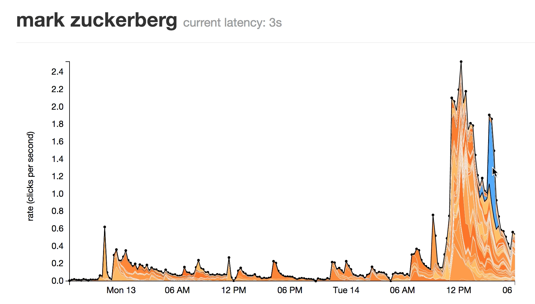
Figure 4. A burst of activity around a phrase in social media
This method allows for a system that can monitor attention to tens of millions of phrases efficiently and in real time.
Finally, some networks have human review before topics are presented publicly to check that they are appropriate. This is a good idea whenever data directly from the Internet is used in a consumer-facing product.
User Segmentation

Figure 5. User are segmented into different groups to understand their behaviours
When operating large websites, it is often important to understand the various types of people that are visiting your pages. This can become quite a task when there are millions of people visiting the website daily and your content is constantly changing. You may be able to do the required analysis overnight, but the result may be of less use the next day; you want to know the types of people visiting the page right now.
This problem highlights the difference between online and offline clustering methods. User segmentation is often done by selecting a group of features from the users’ sessions (for example, the titles or tags of the pages they have gone to and the paths through the website they have taken) and seeing if there are any groups of users who share similar actions. Each of these groups will be considered one cluster and represent one type of user behavior.
One problem, however, is that as the content on your pages changes, so too will the actions of your users. In fact, you could put up a new page that attracts a completely different group of people you have never seen before! It is very useful to be able to understand this right away and see how the changes you make to the content of your website change user behavior in real time.
In a realtime system, we can run an online clustering algorithm which is able to cluster users into distinct populations. As more users perform actions, the characteristics of these populations will change and so will the characterisations given by the clustering algorithm. This allows us to query the algorithm at any point to see if two users are in the same population and how many users are within each group.
Database Precaching
Databases are storing more and more data, which at some point must be stored on a disk or a cluster of disks. As these clusters grow in size, the potential cost for reading from them will invariably increase as well. Some databases try to mitigate this latency through various indexing schemes. An index is a compressed representation of the data with pointers to where you can find the full values.

Figure 6. A quick precaching mechanism reduces the number of requests to the bulky database
For example, riak [4] will store a copy of the index in memory so that we know whether the data even exists and where it is stored. This type of scheme is necessary when we are dealing with potentially very high latency reads from the actual database on disk — if we have a very quick way of first figuring out whether the data exists we can make sure we only do the very expensive disk reads when absolutely necessary.
The riak approach rapidly encounters a problem when the index requires too much memory, however. This can happen very quickly when we want to store many small items. In this case we will quickly fill up memory with all of the keys we are trying to store, even though the actual values do not come close to the storage capacity of our database cluster.
This sort of problem is perfectly suited for a probabilistic data structure. Bloom filters are data structures with a fixed, small memory footprint that store a set of objects and can be queried to see if things are in that set of objects. This allows us to answer the question: for any object, have we seen this object in the past? This question can be answered with no false negatives and only false positives. What this means is that, in the worst-case scenario, a bloom filter will return an incorrect result and say that it has seen an object before when it actually hasn’t (the converse can never happen — a bloom filter will never say it hasn’t seen an object when it really has). In addition, this error can be made incredibly low (in Example 12. Size estimates for the number of unique words in Wikipedia we’ll see that we can store 4,956,262 unique keys with 0.14% error using only 11.5 MB).
By using a bloom filter, we can very easily create a precache that stores all of the keys in the database that we have seen before. If a lookup is requested, we can quickly verify whether we have seen the data before and, if we have, proceed with the expensive disk read. Since we are using a probabilistic data structure for this problem, as opposed to storing the full keyspace in memory, we can store an incredible amount of keys in memory for incredibly fast access while not practically limiting our database capacity to the amount of RAM available. For example, if we wanted our bloom filter to only have a 0.1% error rate, then we could store a representation of 556,421,600 items per gigabyte of RAM (regardless of the actual item size). This is starkly more than the 41,666,666 keys/GB we could store if we stored the raw keys (assuming the keys were 24 characters long and there was no overhead).
This specific problem appears in many places even outside of databases. In biology this approach is frequently used in protein folding problems where backtracking algorithms are used. A small representation of some work that was previously attempted and may have failed can be stored in a probabilistic system so that in future iterations of the algorithm we do not waste time attempting the calculation again. This is particularly important since the actual models that are being worked on are very complex — storing a small representation saves memory and the probabilistic system saves computation so that the algorithm can focus on the folding. This allows the system to perform very large, complex operations and then store a compact representation of the results, which is an efficient way to search through a large, complex space.
In general, whenever calculations are expensive but can be avoided if we can identify whether they’ve been done before, these sorts of precaching algorithms are indispensable.
Graph Databases
The growing interdependencies between systems and groups of people have led to a major focus on graphs as an essential way of understanding the dynamics of social and human networks. Graph techniques have been used in a wide range of applications, from recommendation algorithms (collaborative filtering and SPEAR) to search indexing (PageRank), social networks (frontrunners, influence tracking), and traffic/networking problems for both computer and physical infrastructure (path detection).
In all of these cases, the amount of data we are tracking is large and is only increasing. For example, in the past social networks used to only change by thousands of connections per day, but now the changes can easily be on the order of thousands per second! These systems are taking in more and more data, and we still want to be able to do the same kinds of complex analysis.
For graphs, one major hurdle in this shift to more data is how to efficiently store the data on a cluster of servers. Not only are we storing some value representing a node on the graph, but we must also store connections to other nodes and hopefully be able to retrieve neighboring nodes quickly when necessary. It is this need to constantly be traversing the graph that makes storing graphs difficult. If we have a distributed database and request a user’s data, as well as their friends’ data, the more the information is spread across our cluster the slower our request will be! This is because the most expensive factor in retrieving data from a graph database is the latency in accessing the different nodes in the cluster. It’s much better to make one query to one node than incur large amounts of network overhead getting data from many nodes.
This problem of how to place data in a distributed graph database is called the balanced graph partitioning problem. We want to spread the data onto as many machines and as equally as possible, while minimizing the number of edges that span across machines. A realtime solution to this problem will allow us to start storing truly massive datasets and doing thorough analyses of them where it is currently simply impractical to do so. Currently, most graph databases become impractical once the dataset reaches billions of nodes with a comparable number of relationships. The only remedy that is available is to use considerable resources building customized solutions or using an off-the-shelf solution which has far from optimal performance.
The balanced graph partitioning problem is an open and difficult research problem. A solution to this problem will revolutionize the state of data science.
While there have been many attempts to solve this problem, and there are many promising methods out there, a current leading approach is based on subtree kernels and being able to compare graphs to each other. This problem is quite complex when calculated fully; however, probabilistic methods have been devised that make a fingerprint of the structure of the graph and allow for quick comparisons.

Figure 7. A quick and robust comparison method for graphs opens up completely new analysis possibilities
This method is not only useful as a potential solution to graph partitioning, but also allows us to use graphs for many other applications that were not possible before. We can run classifiers that can classify graphs without having to hand-code features from them. For example, we can compare the types of friend groups (represented as graphs of people) of different people and classify the different communities without having to manually decide what important features in the graph should be considered in the classification. This makes any resulting model much more robust and meaningful, since we can later deduce what features the algorithm thought were important in the classification.
Anomaly Detection
Anomaly detection is another common application. Anomaly detection is akin to finding the needle in the haystack, while other applications that we’ve discussed are more like understanding the nature of the haystack.[5] Furthermore, we want to be able to not only find the needle, but predict when we will next see it and what other haystacks will contain similar needles. In finance, for example, it is critical to be able to find, track, and predict any sort of possible anomalous situation.

Figure 8. Anomaly detection can alert when specific trends start to appear and help correlate multiple signals to eachother
This can become quite taxing computationally as the number of different series of data you are tracking increases. Moreover, when it becomes necessary to correlate different series with one another, the complexity of the system goes through the roof.
Probabilistic data structures and general streaming data analysis can help by filtering out which series possibly have anomalies in them and doing a first-pass correlation in order to reduce the total workload. Various hashing schemes like locality-sensitive hashing provide a quick way to summarize data and find similar instances of it. Furthermore, various methods using HyperLogLog as a first-pass filter have been studied that are able to automatically find correlations within an arbitrary stream of data.
Security and Exploitation
In computer security, it is often hard to be able to identify a threat before it becomes a danger. This is what makes maintaining the security of a network difficult — while it is relatively easy to protect against threats that have been seen before, you never know whether you have already been targeted by new threats. In addition, even if you know the fingerprint of a potential attack, it is often hard to sift through all the requests happening on the network in order to identify it before it is too late.
New measures in computer security focus on identifying trends and patterns in normal service usage and being able to quickly identify when users deviate from the norm. This helps security teams recognize traffic that may represent attack vectors into their systems.
Probabilistic algorithms that are able to summarize the complex traffic pattern of a user — potentially spanning months of service usage — are incredibly important in this process. By being able to summarize these usage patterns and perform similarity measurements on these fingerprints, we are able to quickly spot when something anomalous is happening. In addition, because we’re operating on summaries we can do the calculation quickly and store much less data. This transforms a complex analysis requiring special-purpose hardware into one involving small algorithms that can practically run on routers or load balancers, or concurrently with other services on a system. By being able to do these calculations quickly, we can recognize and prevent intrusions. This will help thwart attacks before they complete instead of identifying them after the fact.
For example, a port scan is when a malicious (or curious) machine attempts many connections to a target server over the network. Algorithms such as thresholded random walks have shown promise at detecting port scans, which have always been hard to monitor because of the low signal-to-noise ratio (for each malicious connection by a port scan there could be thousands of normal connections) and the sheer sophistication of the methods used. With the use of online and probabilistic methods, it is possible to quickly (both computationally and in terms of the number of samples needed) detect port scans with a very low incidence of false negatives.
Algorithms
In this section we present a technical introduction to stream analysis with online algorithms and probabilistic data structures. Then we dive deep into a small selection of probabilistic data structures to give an in-depth understanding of how they work. This understanding of the fundamentals will give the reader a foothold for understanding most of the other probabilistic algorithms in the wild. Finally, we will go through two real-world examples in order to compare the selected data structures.
The source code in this section is presented in the Python programming language, which is commonly used for probabilistic applications and also has the advantage of being easy to read.
This section provides a foundation for actionable decisions regarding which structure to use in different applications.
Realtime Algorithm Primer
Realtime algorithms are generally characterized by being “online” or “one-pass.” This means that the algorithm needs to see a particular piece of data once, and only once, in order to maintain its calculation and later give a response to whatever query the algorithm was designed to answer. While these algorithms generally have a bit more mathematical sophistication, the payoff is an enormous reduction in computation time and memory footprint.
For example, let’s look at two similar algorithms for calculating the variance of a series of numbers. The offline (batch) method would take all of the data points, sum them, and then divide the sum by the total number of data points in order to calculate the mean. Then, we would go back and see how our data points deviated from this mean in order to find the variance. If a new data point came in and we wanted to again know the variance for our dataset, we would need to recalculate the mean and then again go through and see how our data deviates from the new mean.
On the other hand, an online algorithm that calculates the variance for a stream of numbers always maintains the current sum of the data points, how many data points have already been seen, and an auxiliary quantity, M2, that relates to the variance. In this case, whenever we want to know the variance of our dataset we simply must divide the auxiliary quantity that we are maintaining by our count of the number of items. These two quantities that the algorithm keeps track of are called the internal state of the algorithm.
When looking at the complexity of an algorithm, we generally use Big-O notation. In this notation we describe how many operations, in general, the algorithm must perform for an input of length N. For example, if our algorithm is O(N), if we double the amount of data then we double the amount of work that must be done. For O(N^2), a doubling of the data is a quadrupling of the amount of work needed. Ideally an algorithm is O(1), which means the algorithm does not perform differently depending on how much data you give it — it will always have the same performance.
Using these internal states, we are able to shift the computational complexity of a query into the insertion. With the batch algorithm we must do O(1) calculations to insert a new item and O(N) to calculate the average. On the other hand, for the online algorithm we must again do O(1) for an insertion (albeit with a larger constant factor), but only O(1) to calculate the variance! Furthermore, we save on memory as well. For the batch algorithm, we must store every data point we wish to use in our calculation (O(N)); however, the online algorithm only needs to store the two internal state variables (O(1)).
Example 1. Batch versus online variance
class BatchVariance(object):
    # The internal state of this object grows linearly with the amount of data
    # fed into it
    self._dataset = []

    def insert(self, data):
        self._dataset.append(data)

    def mean(self):
        return sum(self._dataset) / float(len(self._dataset))

    def variance(self):
        mean = self.mean()
        exp2 = 0
        for data in self._dataset:
            exp2 += (data - mean)**2
        return exp2 / (n - 1)


class OnlineVariance(object):
    # The internal state of this object is fixed at 3 numbers regardless of how
    # much (or how little) data it has seen
    _n = 0
    _mean = 0
    _M2 = 0

    def insert(self, data):
        self._n += 1
        delta = data - self._mean
        self._mean += delta / self._n
        self._M2 += delta * (data - self._mean)

    def mean(self):
        return self.mean

    def variance(self):
        if self._n < 2:
            return 0
        return self._M2/(self._n - 1)
Online Algorithms for Streams
When working with streaming data, having an online algorithm is critical. It is because we can look at a piece of data once and then throw it away that these algorithms are so attractive. As a result, the computational complexity and memory use of these algorithms are very strictly bounded and they are very well behaved. Batch algorithms, on the other hand, have computational complexity and memory use that are very dependent on the input dataset and can quickly make analysis unfeasible with available hardware and time constraints.
Streams are characterized by a potentially unending sequence of data that is constantly being fed to your algorithms. If your algorithm is online, then the amount of memory required is simply the size of its internal state. For most realtime algorithms (in particular for those described below, except the scaling Bloom filter), the size of the internal state is static and does not depend on how much data has been seen before. That is to say, whether we have just turned on our algorithm or it has been processing data for a month, it will still use the same amount of resources and have the same performance characteristics when processing a query.
Imagine a bucket that can hold any amount of water. That’s an online algorithm. Now imagine a balloon, which expands to hold the amount of water you put inside it. That’s an offline algorithm.
On the other hand, batch algorithms completely depend on how much data they have seen. Many batch algorithms work perfectly well with small amounts of test data but start to under perform when put into production with realistic datasets. This is because as they see more data their internal state grows, which means they not only need to store a larger state but also must process more data every time they respond to a query.
A common remedy for this is to only look at data from a fixed time window (for example, only using the past week’s worth of data). However, this is simply a band-aid for the problem: the algorithm will still do just as poorly if the amount of data seen per day or the complexity of the data increases.[6] Furthermore, these sorts of constraints to the input dataset are often motivated simply by the resource usage of the algorithm and not the actual desired insights from the results, which can result in confusion or simply making the data useless. Most importantly, however, this sort of grouping by time can easily skew statistics. For example, if you were to group your data into hour long groupings, what would happen if you shifted the groups by 30min? How would your insights change if the grouping were changed to 1min instead? This problem stems from the fact that these sorts of models have no optimal value for the number or size of the groupings[7] yet the results are completely dependent on this choice.
Probabilistic Data Structures
Section adapted from High Performance Python by Micha Gorelick and Ian Ozsvald (O’Reilly). Copyright 2014 Micha Gorelick and Ian Ozsvald, 978-1-4493-6159-4.
Probabilistic data structures allow us to make trade-offs in accuracy for immense decreases in memory usage. They are a form of online algorithm that performs a small calculation when data first arrives in order to store a “synopsis” of what it has seen, so it is able to answer queries. As a result, the number of operations we can do on these data structures is much more restricted than when we have the full dataset in a set or a trie. However, with a single HyperLogLog++ structure using 2.56 KB of memory we can count the number of unique items up to approximately 7,900,000,000 items with 1.625% error.
This means that if we were trying to count the number of unique license plate numbers for cars, if our HyperLogLog++ counter said there were 654,192,028, we would be confident that the actual number lies between 664,822,648 and 643,561,407. Furthermore, if this accuracy is not sufficient, we can simply add more memory to the structure and it will perform better. Giving it 40.96 KB of resources will decrease the error from 1.625% to 0.4%. If we had stored the full dataset this would have taken 3.925 GB (and that is assuming no overhead!).
On the other hand, the HyperLogLog++ structure would only be able to count license plates or compare with another collection to see how many license plates the two structures had in common or how many were different. So, for example, we could have one structure for every state in order to find how many unique license plates are in those states. We could then merge them all to get a count for the whole country. However, given a license plate we couldn’t tell you if we’ve seen it before with very good accuracy, and we couldn’t give you a sample of the actual license plate numbers we have already seen. If those were the important questions to ask, we would choose another probabilistic data structure (for example, a Bloom filter) instead.
Probabilistic data structures are fantastic when you have taken the time to understand the problem you are trying to solve and need to put something into production that can answer a very small set of questions about a very large set of data. Each different structure has different questions it can answer at different accuracies, so finding the right one is just a matter of understanding your requirements.
In almost all cases, probabilistic data structures work by finding an alternative representation for the data that is more compact and contains the relevant information for answering a certain set of questions. This can be thought of as a type of lossy compression, where we may lose some aspects of the data but we retain the necessary components. Since we are allowing the loss of data that isn’t necessarily relevant for the particular set of questions we care about, we can still answer the questions at hand while storing the minimal amount of information. It is because of this that the choice of which probabilistic data structure you will use is quite important — you want to pick one that retains the right information for your use case!
Before we dive in, it should be made clear that all the “error rates” here are defined in terms of standard deviations. This term comes from describing Gaussian distributions and describes how spread out a function is around a center value. When the standard deviation grows, so do the number of values further away from the center point. Error rates for probabilistic data structures are framed this way because all the analyses around them are probabilistic. So, for example, when we say that the HyperLogLog algorithm has an error of err = \( \frac{1.04}{\sqrt{m}} \) we mean that 66% of the time the error will be smaller than err, 95% of the time it will be below 2*err, and 99.7% of the time it will be below 3*err. [8]
Very Approximate Counting with a 1-byte Morris Counter
We’ll introduce the topic of probabilistic counting with one of the earliest probabilistic counters, the Morris counter (by Robert Morris of the NSA and Bell Labs). Applications include counting millions of objects in a restricted-RAM environment (e.g., on an embedded computer), understanding large data streams, and problems in AI like image and speech recognition.
The Morris counter keeps track of an exponent and models the counted state as \( 2^{exponent} \) (rather than a correct count) — it provides an order of magnitude estimate. This estimate is updated using a probabilistic rule.
We start with our state, an exponent, set to 0. If we ask for the “value” of the counter, we’ll be given pow(2,exponent) = 1 (the keen reader will note that this is off by one — we did say this was an approximate counter!). If we ask the counter to increment itself it will generate a random number (using the uniform distribution) and test if random(0, 1) <= 1/pow(2,exponent). For exponent == 0 this will always be true and the counter will increment, setting the exponent to 1.
The second time we ask the counter to increment itself it will test if random(0, 1) <= 1/pow(2,1). This will be true 50% of the time. If the test passes, then the exponent is incremented. If not, then the exponent is not incremented for this increment request.
The table below shows the likelihoods of an increment occurring for each of the first exponents.
Table 1. Morris counter details
| exponent | pow(2,exponent) | P(increment) |
|---|---|---|
| 0 | 1 | 1 |
| 1 | 2 | 0.5 |
| 2 | 4 | 0.25 |
| 3 | 8 | 0.125 |
| 4 | 16 | 0.0625 |
| … | … | … |
| 254 | 2.894802e+76 | 3.454467e-77 |
The maximum we could approximately count where we use a single unsigned byte for the exponent is math.pow(2,255) == 5e76. The error relative to the actual count will be fairly large as the counts increase, but the RAM saving is tremendous as we only use 1 byte rather than the 32 unsigned bytes we’d otherwise have to use. In the 1970s, when this scheme was devised, this saving of 31 bytes was tremendous and allowed for previously unimaginable calculations to be done.
Example 2. Simple Morris counter implementation
# A more fully fleshed out implementation which uses an `array` of bytes
# to make many counters is available at:
# https://github.com/ianozsvald/morris_counter

from random import random

class MorrisCounter(object):
    counter = 0
    def add(self, *args):
        if random() < 1.0 / (2 ** self.counter):
            self.counter += 1

    def __len__(self):
        return 2**self.counter
Using the example implementation in Example 2. Simple Morris counter implementation, we can see that the first request to increment the counter succeeds and the second fails. [9]
Example 3. Morris counter library example
In [2]: mc = MorrisCounter()
In [3]: print len(mc)
1.0
In [4]: mc.add()  # P(1) of doing an add
In [5]: print len(mc)
2.0
In [6]: mc.add()  # P(0.5) of doing an add
In [7]: print len(mc)  # the add does not occur on this attempt
2.0
In Figure 1. Three 1-byte Morris counters vs. an 8-byte integer, the thick black line shows a normal integer incrementing on each iteration. On a 64-bit computer this is an 8-byte integer. [10] The evolution of three 1-byte Morris counters is shown as dotted lines: the y-axis shows their values, which approximately represent the true count for each iteration. Three counters are shown to give you an idea about their different trajectories and the overall trend; the three counters are entirely independent of each other.

Figure 1. Three 1-byte Morris counters vs. an 8-byte integer
K-Min Values
When comparing sets is critical — for example, when creating similarity graphs showing connectivity between different communities (such as in the prototype, CliqueStream) or comparing user trends — K-Min Values is the perfect data structure to use.
In the Morris counter, we lose any sort of information about the items we insert. That is to say, the counter’s internal state is the same whether we do .add(“alice”) or .add(“bob”). This extra information is useful and, if used properly, could help us have our counters only count unique items. In this way, calling .add(“alice”) thousands of times would only increase the counter once.
To enable this, we will exploit properties of hashing functions. These functions can be any arbitrary method that takes in an input and assigns a numerical value to it. These values do not need to be unique (in fact, these “collisions” account for most of the error in probabilistic data structures), however they should be repeatable. That is to say, I should get the same result for the same input. However, the main property we would like to take advantage of is the fact that the hash function takes input and uniformly distributes it. For example, let’s assume we have a hash function that takes in a string and outputs a number between 0 and 1. For that function to be uniform means that when we feed it in a string we are equally likely to get a value of 0.5 as a value of 0.2, or any other value. This also means that if we feed it in many string values, we would expect the values to be relatively evenly spaced. Remember, this is a probabilistic argument: they won’t always be evenly spaced, but if we have many strings and try this experiment many times, they will tend to be evenly spaced.
Suppose we took 100 items and stored the hashes of those values (the hashes being numbers from 0-1). Knowing the spacing is even means that instead of saying, “We have 100 items,” we could say, “We have a distance of 0.01 between every item.” This is where the K-Min Values algorithm [11] finally comes in — if we keep the k smallest unique hash values we have seen, we can approximate the overall spacing between hash values and infer what the total number of items is.
In Figure 2. The values stored in a K-Min Values structure as more elements are added we can see the state of a K-Min Values structure (also called a KMV) as more and more items are added. At first, since we don’t have many hash values, the largest hash we have kept is quite large. As we add more and more, the largest of the k hash values we have kept gets smaller and smaller. Using this method, we can get error rates of O\left(\sqrt{\frac{2}{\pi(k-2)}}\right).

Figure 2. The values stored in a K-Min Values structure as more elements are added
This is similar to estimating the number of people in a room by looking at how much space a smaller portion of the group takes up. If we assume that people want to be as spaced out as possible (the property we get from the uniformity of our hash function), then the amount of space k people use indicates the total number of people. For example, if we have a room with a size of 1,000 square feet (sf) and we know that a group of 10 people in the room are taking up 20 sf, then we can estimate there are 500 people in the room!
The larger k is, the more we can account for the hashing function we are using not being completely uniform for our particular input, and for unfortunate hash values. An example of unfortunate hash values would be hashing [“A”, “B”, “C”] and getting the values [0.01, 0.02, 0.03]. If we start hashing more and more values, it is less and less probable that they will clump up.
Furthermore, since we are only keeping the smallest unique hash values, the data structure only considers unique inputs. We can see this easily because if we are in a state where we only store the smallest three hashes and currently [0.1, 0.2, 0.3] are the smallest hash values, if we add in something with the hash value of 0.4 our state will not change. Similarly, if we add more items with a hash value of 0.3, our state will also not change. This is a property called idempotence; it means that if we do the same operation with the same inputs multiple times, the state will not be changed. This is in contrast to, for example, an append on a list, which will always change its value. This concept of idempotence carries on to all of the data structures in this section except for the Morris counter.
Example 4. Simple KMinValues implementation
import mmh3
from blist import sortedset

class KMinValues(object):
    def __init__(self, num_hashes):
        self.num_hashes = num_hashes
        self.data = sortedset()

    def add(self, item):
        item_hash = mmh3.hash(item)
        self.data.add(item_hash)
        if len(self.data) > self.num_hashes:
            self.data.pop()

    def __len__(self):
        if len(self.data) <= 2:
            return 0
        # 2**32-1 normalizes the hashes we store since our hash function gives
        # us a number from 0 to 2**21-1 instead of 0 to 1
        return (self.num_hashes - 1) * (2**32-1) / float(self.data[-2] + 2**31 - 1)
Using the KMinValues implementation in the Python package CountMeMaybe, [12] we can begin to see the utility of this data structure. This implementation is very similar to the one in Example 4. Simple KMinValues implementation, but it fully implements the other set operations, such as union and intersection. Also note that “size” and “cardinality” are used interchangeably (the word “cardinality” is from set theory and is used more in the analysis of probabilistic data structures). Here, we can see that even with a reasonably small value for k, we can store 50,000 items and calculate the cardinality of many set operations with relatively low error:
>>> from countmemaybe import KMinValues

>>> kmv1 = KMinValues(k=1024)

>>> kmv2 = KMinValues(k=1024)

>>> for i in xrange(0,50000): # We put 50,000 elements into kmv1.
    kmv1.add(str(i))
   ...:

>>> for i in xrange(25000, 75000): # kmv2 also gets 50,000 elements, 25,000 of which are the same as those in kmv1
    kmv2.add(str(i))
   ...:

>>> print len(kmv1)
50416

>>> print len(kmv2)
52439

>>> print kmv1.cardinality_intersection(kmv2)
25900.2862992

>>> print kmv1.cardinality_union(kmv2)
75346.2874158
With these sorts of algorithms, the choice of hash function can have a drastic effect on the quality of the estimates. Both of these implementations use mmh3, a Python implementation of mumurhash3 that has nice properties for hashing strings. However, different hash functions could be used if they are more convenient for your particular dataset.
Bloom Filters

Figure 3. Bloom filter
Bloom filters excel at easily distinguishing if a particular item has been seen before. In addition, advanced versions of the algorithms give extra features like scalability and time windowing. This can be useful when making a caching layer or when simply asking whether you have seen a particular user within a certain amount of time.
Sometimes we need to be able to do other types of set operations, for which we need to introduce new types of probabilistic data structures. Bloom filters [13] were created to answer the question of whether we’ve seen an item before.
Bloom filters work by having multiple hash values in order to represent a value as multiple integers. If we later see something with the same set of integers, we can be reasonably confident that it is the same value.
In order to do this in a way that efficiently utilizes available resources, we implicitly encode the integers as the indexes of a list. This could be thought of as a list of bool values that are initially set to False. If we are asked to add an object with hash values [10, 4, 7], then we set the tenth, fourth, and seventh indexes of the list to True. In the future, if we are asked if we have seen a particular item before, we simply find its hash values and check if all the corresponding spots in the bool list are set to True.
This method gives us no false negatives and a controllable rate of false positives. What this means is that if the Bloom filter says we have not seen an item before, then we can be 100% sure that we haven’t seen the item before. On the other hand, if the Bloom filter states that we have seen an item before, then there is a probability that we actually have not and we are simply seeing an erroneous result. This erroneous result comes from the fact that we will have hash collisions, and sometimes the hash values for two objects will be the same even if the objects themselves are not the same. However, in practice Bloom filters are set to have error rates below 0.5%, so this error can be acceptable.
We can simulate having as many hash functions as we want simply by having two hash functions that are independent of each other. This method is called “double hashing.” If we have a hash function that gives us two independent hashes, we can do:
def multi_hash(key, num_hashes):
    hash1, hash2 = hashfunction(key)
    for i in xrange(num_hashes):
        yield (hash1 + i * hash2) % (2^32 - 1)
The modulo ensures that the resulting hash values are 32 bit (we would modulo by 2^64 - 1 for 64-bit hash functions).
The exact length of the bool list and the number of hash values per item we need will be fixed based on the capacity and the error rate we require. With some reasonably simple statistical arguments [14] we see that the ideal values are:
\begin{array} {rcl} num\_bits & = & -capacity \cdot \frac{log(error)}{log(2)^2} \\ num\_hashes & = & num\_bits \cdot \frac{log(2)}{capacity} \end{array}
That is to say, if we wish to store 50,000 objects (no matter how big the objects themselves are) at a false positive rate of 0.05% (that is to say, 0.05% of the times we say we have seen an object before, we actually have not), it would require 791,015 bits (0.7Mb) of storage and 11 hash functions.
To further improve our efficiency in terms of memory use, we can use single bits to represent the bool values (a native bool actually takes 4 bits). We can do this easily by using the bitarray module.
Example 5. Simple Bloom filter implementation
import bitarray
import math
import mmh3

class BloomFilter(object):
    def __init__(self, capacity, error=0.005):
        """
        Initialize a bloom filter with given capacity and false positive rate
        """
        self.capacity = capacity
        self.error = error
        self.num_bits = int(-capacity * math.log(error) / math.log(2)**2) + 1
        self.num_hashes = int(self.num_bits * math.log(2) / float(capacity)) + 1
        self.data = bitarray.bitarray(self.num_bits)

    def _indexes(self, key):
        h1, h2 = mmh3.hash64(key)
        for i in xrange(self.num_hashes):
            yield (h1 + i * h2) % self.num_bits

    def add(self, key):
        for index in self._indexes(key):
            self.data[index] = True

    def __contains__(self, key):
        return all(self.data[index] for index in self._indexes(key))

    def __len__(self):
        num_bits_on = self.data.count(True)
        return -1.0 * self.num_bits * math.log(1.0 - num_bits_on / float(self.num_bits)) / float(self.num_hashes)

    @staticmethod
    def union(bloom_a, bloom_b):
        assert bloom_a.capacity == bloom_b.capacity, "Capacities must be equal"
        assert bloom_a.error == bloom_b.error, "Error rates must be equal"

        bloom_union = BloomFilter(bloom_a.capacity, bloom_a.error)
        bloom_union.data = bloom_a.data | bloom_b.data
        return bloom_union
What happens if we insert more items than we specified for the capacity of the Bloom filter? At the extreme end, all the items in the bool list will be set to True, in which case we say that we have seen every item. This means that Bloom filters are very sensitive to what their initial capacity was set to, which can be quite aggravating if we are dealing with a set of data whose size is unknown (for example, a stream of data).
One way of dealing with this is to use a variant of Bloom filters called scalable Bloom filters. [15] They work by chaining together multiple Bloom filters whose error rates vary in a specific way. [16] By doing this, we can guarantee an overall error rate and simply add a new Bloom filter when we need more capacity. In order to check if we’ve seen an item before, we simply iterate over all of the sub-Blooms until either we find the object or we exhaust the list. A sample implementation of this structure can be seen in Example 6. Simple scaling Bloom filter implementation, where we use the previous Bloom filter implementation for the underlying functionality and have a counter to simplify knowing when to add a new Bloom.
Another way of dealing with this is using a method called timing Bloom filters. [17] This variant allows elements to be expired out of the data structure, thus freeing up space for more elements. This is especially nice for dealing with streams, since we can have elements expire after, say, an hour and have the capacity be large enough to deal with the amount of data we see per hour. Using a Bloom filter this way would give us a nice view into what has been happening in the last hour.
Example 6. Simple scaling Bloom filter implementation
from bloomfilter import BloomFilter

class ScalingBloomFilter(object):
    def __init__(self, capacity, error=0.005, max_fill=0.8, error_tightening_ratio=0.5):
        self.capacity = capacity
        self.base_error = error
        self.max_fill = max_fill
        self.items_until_scale = int(capacity * max_fill)
        self.error_tightening_ratio = error_tightening_ratio
        self.bloom_filters = []
        self.current_bloom = None
        self._add_bloom()

    def _add_bloom(self):
        new_error = self.base_error * self.error_tightening_ratio ** len(self.bloom_filters)
        new_bloom = BloomFilter(self.capacity, new_error)
        self.bloom_filters.append(new_bloom)
        self.current_bloom = new_bloom
        return new_bloom

    def add(self, key):
        if key in self:
            return True
        self.current_bloom.add(key)
        self.items_until_scale -= 1
        if self.items_until_scale == 0:
            bloom_size = len(self.current_bloom)
            bloom_max_capacity = int(self.current_bloom.capacity * self.max_fill)

            # We may have been adding many duplicate values into the bloom, so
            # we need to check if we actually need to scale or if we still have
            # space
            if bloom_size >= bloom_max_capacity:
                self._add_bloom()
                self.items_until_scale = bloom_max_capacity
            else:
                self.items_until_scale = int(bloom_max_capacity - bloom_size)
        return False

    def __contains__(self, key):
        return any(key in bloom for bloom in self.bloom_filters)

    def __len__(self):
        return sum(len(bloom) for bloom in self.bloom_filters)
Using this data structure will feel much like using a set object. Below we use a scalable Bloom filter to add several objects, test if we’ve seen them before, and then try to experimentally find the false positive rate:
>>> bloom = BloomFilter(100)

>>> for i in xrange(50):
   ....:     bloom.add(str(i))
   ....:

>>> "20" in bloom
True

>>> "25" in bloom
True

>>> "51" in bloom
False

>>> num_false_positives = 0

>>> num_true_negatives = 0

>>> # None of the following numbers should be in the Bloom.
>>> # If one is found in the Bloom, it is a false positive.
>>> for i in xrange(51,10000):
   ....:     if str(i) in bloom:
   ....:         num_false_positives += 1
   ....:     else:
   ....:         num_true_negatives += 1
   ....:

>>> num_false_positives
54

>>> num_true_negatives
9895

>>> false_positive_rate = num_false_positives / float(10000 - 51)

>>> false_positive_rate
0.005427681173987335

>>> bloom.error
0.005
We can also do unions with Bloom filters in order to join multiple sets of items. One caveat with this is that you can only take the union of two Blooms with the same capacity and error rate. Furthermore, the final Bloom’s used capacity can be as high as the sum of the used capacities of the two Blooms unioned to make it. What this means is that you could start with two Bloom filters that are a little more than half full and, when you union them together, get a new Bloom that is over capacity and not reliable!
>>> bloom_a = BloomFilter(200)

>>> bloom_b = BloomFilter(200)

>>> for i in xrange(50):
   ...:     bloom_a.add(str(i))
   ...:

>>> for i in xrange(25,75):
   ...:     bloom_b.add(str(i))
   ...:

>>> bloom = BloomFilter.union(bloom_a, bloom_b)

>>> "51" in bloom_a # <1>
Out[9]: False

>>> "24" in bloom_b # <2>
Out[10]: False

>>> "55" in bloom # <3>
Out[11]: True

>>> "25" in bloom
Out[12]: True
-
The value of “51” is not in bloom_a.
-
Similarly, the value of “24” is not in bloom_b.
-
However, the bloom object contains all the objects in both bloom_a and bloom_b!
LogLog Counters
LogLog counters, particularly HyperLogLog++, offer the best efficiency when counting the size of a set or taking the union of sets. They don’t, however, do well at intersections. They can be useful, for example, when counting unique users by geography and allowing for accumulations based on different geographic combinations. In general, LogLog-type algorithms are very versatile, and there are even adaptations that can temporally window your data.
LogLog-type counters [18] are based on the realization that the individual bits of a hash function can also be considered to be random. That is to say, the probability of the first bit of a hash being 1 is 50%, the probability of the first two bits being 01 is 25%, and the probability of the first three bits being 001 is 12.5%. Knowing these probabilities, and keeping the hash with the most 0s at the beginning (i.e., the least probable hash value), we can come up with an estimate of how many items we’ve seen so far.
A good analogy for this method is flipping coins. Imagine we would like to flip a coin 32 times and get heads every time. The number 32 comes from the fact that we are using 32-bit hash functions. If we flip the coin once and it comes up tails, then we will store the number 0, since our best attempt yielded 0 heads in a row. Since we know the probabilities behind this coin flip, we can also tell you that our longest series was 0 long and you can estimate that we’ve tried this experiment 2^0 = 1 time. If we keep flipping the coin and we’re able to get 10 heads before getting a tail, then we would store the number 10. Using the same logic, you could estimate that we’ve tried the experiment 2^10 = 1024 times. With this system, the highest we could count would be the maximum number of flips we consider (for 32 flips, this is 2^32 = 4,294,967,296).
In order to encode this logic with LogLog-type counters, we take the binary representation of the hash value of our input and see how many 0 s there are before we see our first 1. The hash value can be thought of as a series of 32 coin flips, where 0 means a flip for heads and 1 means a flip for tails (i.e., 000010101101 means we flipped 4 heads before our first tails and 010101101 means we flipped 1 head before flipping our first tail). This gives us an idea of how many attempts happened before this hash value was gotten. The mathematics behind this system are almost equivalent to those of the Morris counter, with one major exception: the “random” values are acquired by looking at the actual input instead of using a random number generator. This means that if we keep adding the same value to a LogLog counter its internal state will not change.
Example 7. Simple implementation of LogLog register
import mmh3

def trailing_zeros(number):
    """
    Returns the index of the first bit set to 1 from the right side of a 32-bit
    integer
    >>> trailing_zeros(0)
    32
    >>> trailing_zeros(0b1000)
    3
    >>> trailing_zeros(0b10000000)
    7
    """
    if not number:
        return 32
    index = 0
    while (number >> index) & 1 == 0:
        index += 1
    return index

class LogLogRegister(object):
    counter = 0
    def add(self, item):
        item_hash = mmh3.hash(str(item))
        return self._add(item_hash)

    def _add(self, item_hash):
        bit_index = trailing_zeros(item_hash)
        if bit_index > self.counter:
            self.counter = bit_index

    def __len__(self):
        return 2**self.counter
The biggest drawback of this method is that we may get a hash value that increases the counter right at the beginning and skews our estimates. This would be similar to flipping 32 tails on the first try. In order to remedy this, we should have many people flipping coins at the same time and combine their results. The law of large numbers tells us that as we add more and more flippers, the total statistics become less affected by anomalous samples from individual flippers. The exact way that we combine the results is the root of the difference between LogLog-type methods (classic LogLog, SuperLogLog, HyperLogLog, HyperLogLog++, etc.).
This “multiple flipper” method can be accomplished by taking the first couple of bits of a hash value and using that to designate which of our flippers had that particular result. If we take the first 4 bits of the hash, this means we have 2^4 = 16 flippers. Since we used the first 4 bits for this selection, we only have 28 bits left (corresponding to 28 individual coin flips per coin flipper), meaning each counter can only count up to 2^28 = 268,435,456. In addition, there is a constant (alpha) that depends on the number of flippers there are, which normalizes the estimation. [19] All of this together gives us an algorithm with \( \frac{1.05}{\sqrt{m}} \) accuracy, where m is the number of registers (or flippers) used.
Example 8. Simple implementation of LogLog
from llregister import LLRegister
import mmh3

class LL(object):
    def __init__(self, p):
        self.p = p
        self.num_registers = 2**p
        self.registers = [LLRegister() for i in xrange(int(2**p))]
        self.alpha = 0.7213 / (1.0 + 1.079 / self.num_registers)

    def add(self, item):
        item_hash = mmh3.hash(str(item))
        register_index = item_hash & (self.num_registers - 1)
        register_hash = item_hash >> self.p
        self.registers[register_index]._add(register_hash)

    def __len__(self):
        register_sum = sum(h.counter for h in self.registers)
        return 2 ** (float(register_sum) / self.num_registers) * self.num_registers * self.alpha
In the __len__ method, we are averaging the estimates from all of the individual LogLog registers. This, however, is not the most efficient way to combine the data! This is because we may get some unfortunate hash values that make one particular register spike up while the others are still at low values. Because of this, we are only able to achieve an error rate of \( O ( \frac{1.30}{\sqrt{m}} ) \), where m is the number of registers used.
SuperLogLog [20] was devised as a fix to this problem. With this algorithm, only the lowest 70% of the registers were used for the size estimate, and their value was limited by a maximum value given by a restriction rule. This addition decreased the error rate to \( O(\frac{1.05}{\sqrt{m}}) \). This was counterintuitive, since we got a better estimate by disregarding information!
Finally, HyperLogLog [21] came out in 2007 and gave us further accuracy gains. This was done simply by changing the method of averaging the individual registers: instead of simply averaging, we use a spherical averaging scheme [22] that also has special considerations for different edge cases the structure could be in. This brings us to the current best error rate of \( O(\frac{1.04}{\sqrt{m}}) \). In addition, this formulation removes a sorting operation that is necessary with SuperLogLog. This can greatly speed up the performance of the data structure when trying to insert items at a high volume.
Example 9. Simple implementation of HyperLogLog
# the following import imports our previously defined LogLog register
from ll import LL
import math

class HyperLogLog(LL):
    def __len__(self):
        indicator = sum(2**-m.counter for m in self.registers)
        E = self.alpha * (self.num_registers**2) / float(indicator)

        if E <= 5.0 / 2.0 * self.num_registers:
            V = sum(1 for m in self.registers if m.counter == 0)
            if V != 0:
                Estar = self.num_registers * math.log(self.num_registers / (1.0 * V), 2)
            else:
                Estar = E
        else:
            if E <= 2**32 / 30.0:
                Estar = E
            else:
                Estar = -2**32 * math.log(1 - E / 2**32, 2)
        return Estar

if __name__ == "__main__":
    import mmh3
    hll = HyperLogLog(8)
    for i in xrange(100000):
        hll.add(mmh3.hash(str(i)))
    print len(hll)
The only further increase in accuracy was given by the HyperLogLog++ algorithm, which increased the accuracy of the data structure while it is relatively empty. When more items are inserted, this scheme reverts to standard HyperLogLog. This is actually quite useful, since the statistics of the LogLog-type counters require a lot of data to be accurate — having a scheme for allowing better accuracy with fewer items greatly improves the usability of this method. This extra accuracy is achieved by having a smaller but more accurate HyperLogLog structure that can be later converted into the larger structure that was originally requested. Also, there are some imperially derived constants that are used in the size estimates that remove biases.
Composite Structures
It is important to note that the above structures are simply the building blocks for more complicated algorithms and methods. We can put these tools together in different ways in order to achieve various results.
For example, one common problem we chose to solve in the prototype was identifying which of several thousand phrases occurs within a given piece of text. To make matters worse, this calculation needed to happen very quickly, since we were parsing many messages per second.
The resulting solution was a hierarchy of Bloom filters arranged in such a way as to efficiently implement a Rabin–Karp string search algorithm. This gave us the low memory use of a Bloom filter and the efficiency of an optimized string searching algorithm. In the end, we were able to search through 1,000 words for one of 16,000 variable-length keywords in under a millisecond on commodity hardware.
from bloomfilter import BloomFilter
from itertools import ifilter


class MultigramSearch(object):
    def __init__( self, ngrams, delimiter='##', stop='$$',
            error=0.0001, error_tightening_ratio=0.5):
        self.blooms = []
        self.error = error
        self.error_tightening_ratio = error_tightening_ratio
        self.min_ngram = min(len(d) for d in ngrams) or 1
        self.max_ngram = max(len(d) for d in ngrams)
        self.delimiter = delimiter
        self.STOP = stop
        self._build_structure(ngrams)

    def _build_structure(self, ngrams):
        delimiter = self.delimiter
        STOP = self.STOP
        for i, n in enumerate(xrange(self.min_ngram, self.max_ngram+1)):
            num_items = sum(1 for x in ngrams if len(x) >= n)
            # we tighten the error so that the compounded error converges to
            # the desired error
            cur_error = self.error * (self.error_tightening_ratio ** i)
            bloom = BloomFilter(num_items, error=cur_error)
            for item in ifilter(None, ngrams):
                if len(item) >= n:
                    bloom.add(delimiter.join(item[:n]))
                elif len(item) + 1 == n:
                    bloom.add(delimiter.join(item) + STOP)
            self.blooms.append(bloom)

    def intersection(self, text):
        i = 0
        offset = self.min_ngram
        L = len(text) - offset
        delimiter = self.delimiter
        while i <= L:
            for N, bloom in enumerate(self.blooms):
                # check if the current substring is in the bloom filter without
                # the STOP sequence -- this would mean we have a partial ngram
                # match
                test = delimiter.join(text[i:i+N+offset])
                if test not in bloom:
                    if N > 0:
                        # now we check if the current bloom has the substring
                        # with the STOP sequence appended to it
                        new_test = delimiter.join(text[i:i+N+offset-1])
                        if (new_test + self.STOP) in bloom:
                            yield text[i:i+N+offset-1]
                    break
            i += N + 1
Real-World Example
For a better understanding of the data structures, we first created a dataset with many unique keys, and then one with duplicate entries. Example 10. Comparison between various probabilistic data structures for unique (above) and repeating (below) data shows the results when we feed these keys into the data structures we’ve just looked at and periodically query, “How many unique entries have there been?”
Probabilistic data structures are about guarantees — once you know the questions you’re asking and the computational constraints, you can pick the structure that makes the right guarantees for your situation.
Example 10. Comparison between various probabilistic data structures for unique (above) and repeating (below) data
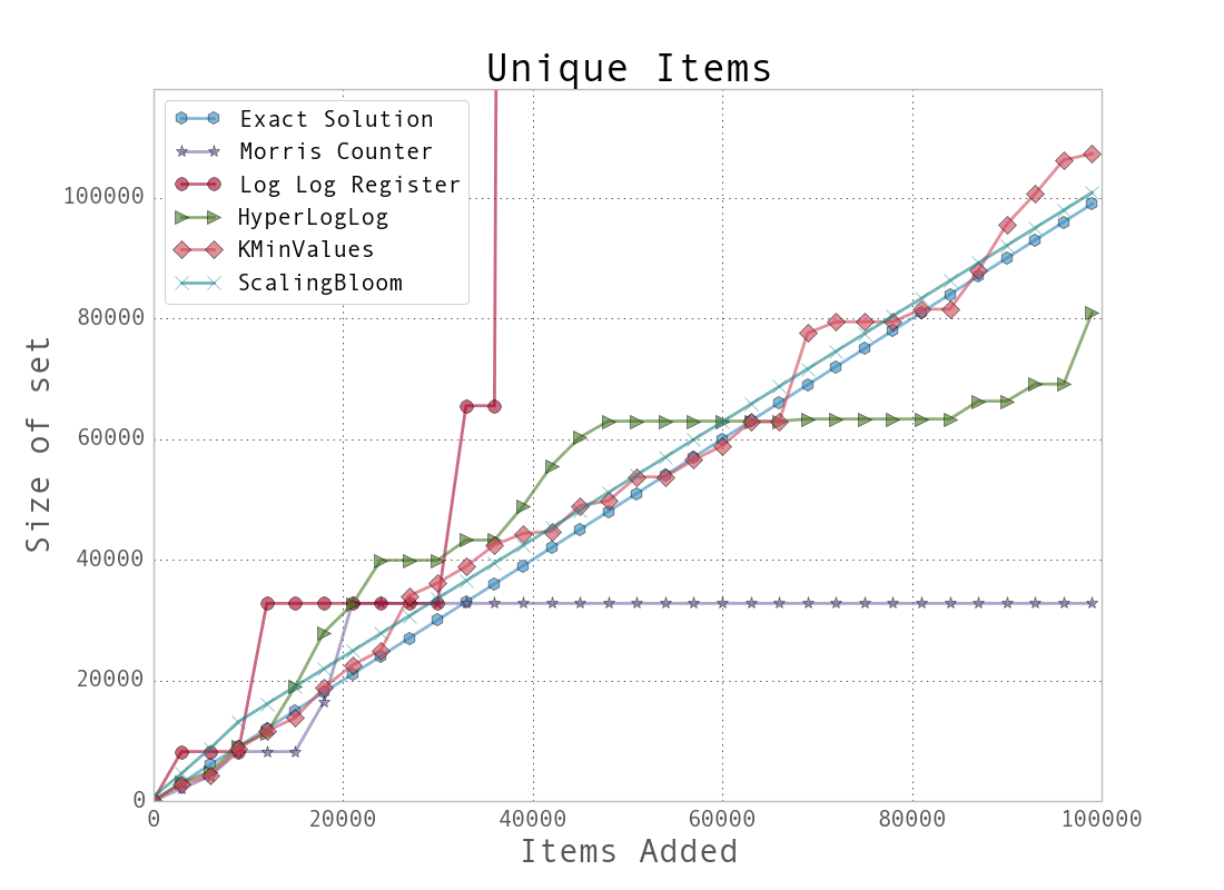
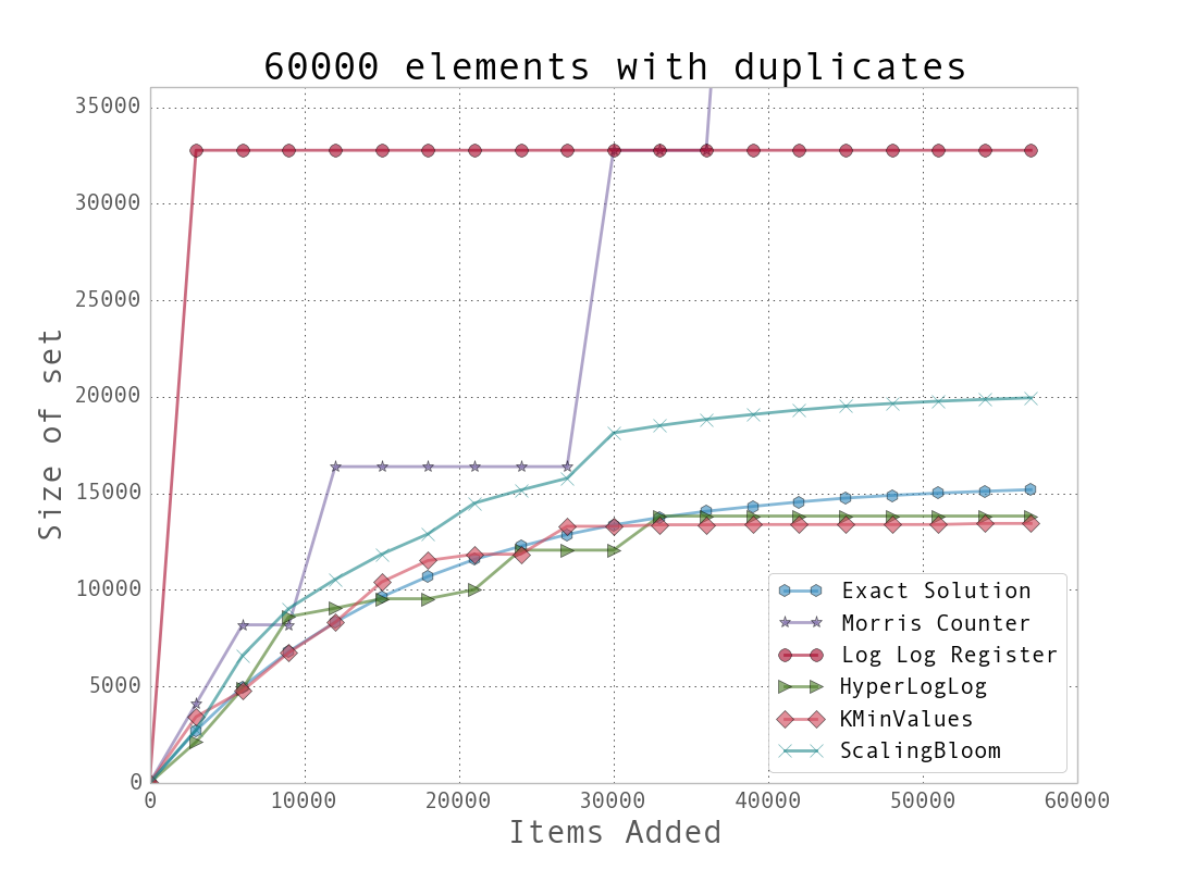
We can see that the data structures that contain more stateful variables (such as HyperLogLog and K-Min Values) do better, since they more robustly handle bad statistics. On the other hand, the Morris counter and the single LogLog register can quickly have very high error rates if one unfortunate random number or hash value occurs. For most of the algorithms, however, we know that the number of stateful variables is directly correlated with the error guarantees, so this makes sense.
Looking just at the probabilistic data structures that have the best performance (and really, the ones you will probably use), we can summarize their utility and their approximate memory usage (see Example 11. Comparison of major probabilistic data structures). We can see a huge change in memory usage depending on the questions we care to ask. This simply highlights the fact that when using a probabilistic data structure, you must first consider what questions you really need to answer about the dataset before proceeding. Also note that only the Bloom filter’s size depends on the number of elements. The HyperLogLog and K-Min Values’s sizes are only dependent on the error rate.
Example 11. Comparison of major probabilistic data structures
| Size | Union [23] | Intersection | Contains | Size [24] | |
|---|---|---|---|---|---|
| HyperLogLog | Yes ( \( O(\frac{1.04}{\sqrt{m}}) \) ) | Yes | No [25] | No | 2.704 MB |
| K-Min Values | Yes ( \( O(\sqrt{\frac{2}{\pi(m-2)}}) \) ) | Yes | Yes | No | 20.372 MB |
| Bloom filter | Yes ( \( O(\frac{0.78}{\sqrt{m}}) \) ) | Yes | No [25] | Yes | 197.8 MB |
As another, more realistic test, we chose to use a dataset derived from the text a partial dump of Wikipedia. This set contains 8,545,076 unique tokens from a portion of the English Wikipedia site and takes up 111 MB on disk. We ran a very simple script in order to extract all single-word tokens with five or more characters from the dataset and store them in a newline-separated file. The question then was, “How many unique tokens are there?” The results can be seen in Example 12. Size estimates for the number of unique words in Wikipedia. In addition, we attempted to answer the same question using a trie structure (this trie was chosen as opposed to the others because it offers good compression while still being robust enough to deal with the entire dataset).
Example 12. Size estimates for the number of unique words in Wikipedia
| Elements | Relative error | Processing time [26] | Structure size [27] | |
|---|---|---|---|---|
| Morris counter [28] | 1,073,741,824 | 6.52% | 751s | 5 bits |
| LogLog register | 1,048,576 | 78.84% | 1,690 s | 5 bit |
| LogLog | 4,522,232 | 8.76% | 2,112 s | 41 KB |
| HyperLogLog | 4,983,171 | -0.54% | 2,907 s | 40 KB |
| K-Min Values | 4,912,818 | 0.88% | 3,503 s | 256 KB |
| Scaling Bloom | 4,949,358 | 0.14% | 10,392 s | 11,509 KB |
| Datrie | 4,505,514 [29] | 0.00% | 14,620 s | 114,068 KB |
| True value | 4,956,262 | 0.00% | ----- | 49,558 KB [30] |
The major takeaway from this experiment is that if you are able to specialize your code, you can get amazing speed and memory gains. Probabilistic data structures are an algorithmic way of specializing your code. We store only the data we need in order to answer specific questions with given error bounds. By only having to deal with a subset of the information given, not only can we make the memory footprint much smaller, but we can also perform most operations over the structure faster (as can be seen with the insertion time into the datrie in Example 12. Size estimates for the number of unique words in Wikipedia being larger than with any of the probabilistic data structures).
As a result, whether or not you use probabilistic data structures, you should always keep in mind what questions you are going to be asking of your data and how you can most effectively store that data in order to ask those specialized questions. This may come down to using one particular type of list over another, using one particular type of database index over another, or maybe even using a probabilistic data structure to throw out all but the relevant data!
CliqueStream: Prototype
The major proliferation of social networks into our communities offers a fantastic opportunity to study the ways in which people interact on a large scale. However, doing so can be quite a computational challenge — many things on the social web are constantly in flux, and there is always new data to consider. In addition, the calculations we wish to perform can often be computationally intensive, to the point where we can no longer easily incorporate all of the newest information into our results. This is what makes analyzing social networks a perfect application for streaming algorithms.
In our prototype, CliqueStream, we wished to create a connected graph including subreddits and Twitter hashtags where the connections are formed by the similarities in the rhetoric used. Furthermore, we wished to be able to identify trends for specific keywords and the similarities between users interacting in these various groups.
This prototype presents a realtime visualization of the relationships between billions of words being used on two major social networks, reddit and Twitter. It allows us to explore current language use and to understand how people are discussing and interacting with new ideas, and the relationships between those ideas. This prototype is both a showcase for the probabilistic methods discussed in this report and a novel visualization of a fascinating data set.
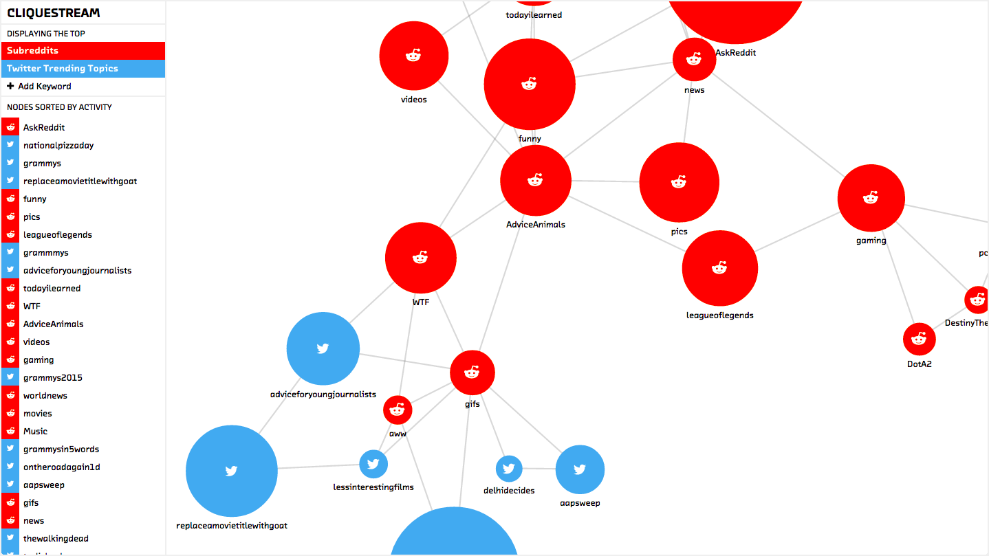
Figure 1. The Cliquestream prototype
All of these calculations can be quite taxing — analyzing the similarity of word use between 50 subreddits can easily result in trillions of comparisons, depending on the number of words used in each one. A classic algorithm for comparing the similarity between two sets results in (N) operations, where N is the number of items the larger of the two sets (this is assuming the data was heavily preprocessed and sorted). If each of the 50 subreddits used 1,000,000 words, then creating this graph would take more than 1,225,000,000 operations! Even if every operation happened in 0.5 microseconds, this would still amount to 10.2 minutes of computation.
On the other hand, if we used a probabilistic data structure (such as a K-Min Values structure with 1.75% error), we could reduce the number of operations to 2,508,800. This would represent 1.25 seconds of work, as compared to 10.2 minutes for the classical computation. The ability to do this calculation quickly allows us to create an informative and interactive frontend where users can play with data and get results immediately. As a result, instead of us pre-describing what we want our users to see, they can form their own complicated queries and see the results right away.
Don’t underestimate the power of responsive data analysis. If an analyst must wait a 10 minutes for a result instead of seconds, there’s a psychological cost to the context switch that slows down the human part of the creative data analysis process.
Probabilistic algorithms sped up our analysis by 490x, making it possible for results to be computed in real time.
In addition to the savings in computation, writing our algorithms probabilistically gave us an enormous savings in memory used. As described in algorithms, analyzing data probabilistically allows us to store only a small synopsis of the data as opposed to the full dataset. This is particularly useful when dealing with a stream of data, where storing the full dataset would constantly require more and more storage space. Our probabilistic implementation has bounded memory use — once enough subreddit and hashtag data comes in to fill the data structures with the minimum amount of data necessary (see Things to Consider for more discussion), the memory use stabilizes. In the case of our prototype this stabilization happens at 296.3 MB of memory and 147 MB of storage (including data snapshots for reloading the in-memory data). This is quite amazing considering we are ingesting data at a rate of 1.59 Mb/s (with a modest 40 messages per second) and see a gigabyte of data every hour and a half!
The ability to bound our memory use and our computational complexity also saves us maintenance time and decreases system complexity. Our prototype easily runs on any standard laptop, yet it delivers the kind of results that are generally associated with a cluster solution (Hadoop, for example) that requires extraordinary computing power and significant manpower to maintain.
Implementation
An important aspect when designing a good data analysis pipeline with streams is to decouple as many of the components from each other as possible. That is to say, the various elements should communicate through a simple API and not be dependent on their particular implementation. This is a strong principle of modern system architecture and is particularly relevant for stream-based systems.

Figure 2. General streaming data analysis pipeline
This decoupling is beneficial because it allows developers to work concurrently without affecting each other’s systems. In addition, if the interface is sufficiently general (for example, using an HTTP-based API), then individual developers can use any language in order to implement a particular segment of the overall system.
Furthermore, scaling becomes much easier when the components are modular. If we start by running the entire system on one server and soon realize we need more computing power or better fault tolerance, we can move some of the system to new servers that can function as backup systems or provide additional computational capacity.
In general, the components of a data processing pipeline involve gathering the data, moving the data to the right places, analyzing it, and providing a method to gather the results. In classic batch infrastructures (such as Hadoop), the results are provided in a text file that contains the output of the analysis. For a streaming architecture, we need a way to query the system whenever we want to see what the current state of the calculation is. To accommodate this, we chose to create a REST API such that any external system can issue queries to the system and see what the current results are. Alternatively, some analysis schemes can provide new, modified versions, of the original data stream for other processes to take advantage of. Generally this is used to either filter the stream (by removing non-pertinent messages) or to augment it (by adding new fields).
For example, in Figure 2. General streaming data analysis pipeline the cat_extractor analysis routine finds tweets relating to cats and filters them into their own stream (named the cat_stream). Any other analysis routine can now read this filtered stream and do further analysis to it (such at the all_cat_tweets routine).
Components of a Processing Pipeline
-
Data Sources
- Data Source-Specific Libraries
-
Data Routing
-
NSQ
-
RabbitMQ
-
Kafka
-
Amazon Kinesis
-
-
Analysis Plugins
-
Any Language
-
Simple and Uniform API
-
-
Query Interface
- REST API
Collection and Analysis Pipeline
The first hurdle when working with streaming data is setting up an infrastructure that can route messages to the correct place. This can be made even more challenging when dealing with multiple sources of data, some of which support streaming and some of which require polling.
For the prototype, we identified two main data sources of interest: reddit and Twitter. The Twitter API supports streaming results. For this, we regularly check which hashtags are currently trending and set up a stream of tweets that mention these entities. This provides our backend with a constant supply of data to parse.
Reddit, on the other hand, requires that our backend go and fetch new data at regular intervals. This was set up as an asynchronous process that gets new data and fills a buffer with it. Once the buffer is full, we can process this data.
For this particular prototype, we chose to have the code generating the data speak directly to the analysis plugins. However, for more complicated situations (e.g., when multiple different systems need access to the same stream of data), a messaging protocol should be used. NSQ [31] is a simple solution that does just that — data can be published to different topics and consumers can subscribe to those topics in order to read the stream. These sorts of systems also help deal with fault tolerance by having guarantees on the delivery of each message. Furthermore, they allow for easy scaling of a system by decoupling systems from each other (see “NSQ for Robust Production Clustering” in Chapter 10 of High Performance Python for a more in-depth discussion).
As data is coming in, we queue it into small batches. This idea of mini-batches (approximately 50-100 messages per batch) is incredibly important when doing performance analysis. While our algorithms are online and can handle one piece of data at a time, we can greatly optimize the I/O performance by handling small batches. It is quite important to tune any I/O, whether it is an API request or a database operation or simply updating an in-memory data structure, such that the overhead of initializing such an operation is offset by the amount of work that is actually done (see Chapter 8 of High Performance Python for a more in-depth treatment of this issue).
An example of using mini-batches is with making API requests through an HTTP interface. If we were requesting data for 50 different users, we could either initiate 50 different requests or use an endpoint that can satisfy all requests for us at once. While the total amount of data being transferred back and forth is the same, we expect the batched request to complete faster since we only need to initiate one HTTP connection. This speedup is most evident when the time to transfer the actual response data becomes comparable to the time to initialize a connection.
The batches of data are sent to a collection of processing plugins. These plugins do a variety of things, from maintaining the probabilistic data structures to checking the health of the system. The only requirement is that the plugin inherits from the PluginBase object to ensure we can properly maintain the state and integrity of the pipeline.
class PluginBase(object):
    def save(self, location):
        """
        Save the current state of the plugin to the directory location
        """
        logger.info("Save not implemented")

    def load(self, location):
        """
        Load state from directory location or raise exception
        """
        logger.info("Load not implemented")

    def __call__(self, messages):
        """
        Process messages in the messages list. Raise exception on fatal error
        that should stop processing.
        """
        logger.info("Call not implemented")

    def routes(self):
        """
        Return description of the HTTP routes in order to get plugin state. For
        example, we could return the following list of tuples to register
        "plugin/get" and "plugin/status":
            [
                ('/plugin/get'    , GetHandler)    ,
                ('/plugin/status' , StatusHandler) ,
            ]
        The handler objects should inherit from tornado.web.BaseHandler.
        """
        logger.info("Routes not implemented")
These plugins are all responsible for their own external APIs (as defined by their routes functionality). Therefore, each plugin can register as many interfaces into its state as are necessary. This allows us to create multiple routes for each plugin in order to get different insights into the analyses they are performing. For example, our plugin that handles tracking the words used in a subreddit/hashtag registers one route to find the number of unique words used in that community and another route to compare the similarity of multiple communities.
Comparing Words
To calculate the similarity between word choices, we used a K-Min Values data structure with k set to 1024 (see kminvalues). This choice was made because this structure can efficiently calculate the Jaccard distance between two sets, which encodes how similar they are normalized by how big they are. This is the perfect score for quantifying how much two subreddits or hashtags share word usage while normalizing for particularly verbose communities.
The implementation was done in GoLang and is called gocountme [32] it provides a simple HTTP interface to manipulate probabilistic sets. This allows us to very simply add elements to a collection and then do various set operations on them. For example, we can easily add all users of a website and compare them in a language-agnostic way.
$ for user in $( cat site_A_users.txt ); do
    curl "http://gocountme/add?key=siteA&value=${user}";
done;

$ for user in $( cat site_B_users.txt ); do
    curl "http://gocountme/add?key=siteB&value=${user}";
done;

$ curl "http://gocountme/cardinality?key=siteA"
{
  "status_code": 200,
  "status_txt": "",
  "data": 9943.261918592398 # Actual cardinality is 10,000 (an error of 0.56%)
}

$ curl "http://gocountme/correlation?key=siteA&key=siteB"
{
  "status_code": 200,
  "status_txt": "",
  "data": [
    {
      "keys": [
        "siteA",
        "siteB"
      ],
      "jaccard": 0.234375 # Actual Jaccard distance is 0.2305 (an error of 1.65%)
    }
  ]
}
This system was engineered to optimize for throughput and availability by using Google’s leveldb [33] library. In addition, it supports writing customized queries through a simple querying language in order to build up complicated statements that can easily be evaluated server-side.
Lastly, we can examine the actual state of the internal K-Min Values structure. This allows us to easily accumulate data from multiple gocountme instances and perform calculations on them — so, we can have small gocountme instances on many computers in order to maintain local statistics with the ability to accumulate the states to gather insights into global statistics.
Keyword Usage
Keyword monitoring requires solving two problems: first we must be able to efficiently extract valuable keywords from a given text, and then we must be able to maintain relevant statistics for them. Extracting keywords can quickly become a difficult problem as the number of keywords being tracked increases. Likewise, maintaining statistics for that set can become difficult as we start wanting to store statistics for hundreds of thousands of items.
In order to extract the keywords from a text, we use the hierarchical Bloom filter described in Composite Structures. This allows us to find any of 10,000 keywords using only 56.7 KB of memory. Simply storing the keywords in a hash table for lookup would require 2192.8 KB; however, considerably more space would be required to efficiently search for the keywords within a text, since a lot of preprocessing must be done. Furthermore, the Bloom filter’s memory use is agnostic to the actual size of the keywords and only scales with the number of them.
Once we have extracted the keyword data, we insert an association of subreddit/hashtag to keyword into a system called forgettable. [34] At first look, forgettable seems to simply be a database for categorical distributions — it can store the counts and probabilities of keyword mentions for each subreddit or hashtag. However, it uses a scheme borrowed from radioactive decay using Poisson processes in order to discard old data and slowly “forget” old statistics.

Figure 3. Different results with different data expiration policies
The ability to forget old data in this way gives us many advantages. Firstly, we can bound the size of the database so that we aren’t constantly required to upgrade the server’s capacity. Also, we are able to discard old data without having to store information regarding when the data first came in or having discontinuities in our data as a result of data expiration policies.
Storing timestamps for when data was inserted can be quite a burden on a data store. In fact, storing data insertion times for the purpose of deleting old data can easily grow the size of your data by many orders of magnitude. In addition to the extra storage comes the extra computation necessary to sift through the metadata in order to find the correct elements to delete. This method has also been implemented in the past by inserting data into a queue (thus avoiding the need to store additional timestamps); however, this organization of the data greatly reduces the speed of the system by forcing a complete recalculation of results at every query.
Alternatively, another common scheme for forgetting data is to “expire” it (i.e., delete it from the database completely after a certain period). However, this causes problems with the statistics: old data does not fade away into the background, but rather all the data simply disappears after a certain time, causing discontinuities in any insights given from the data.
With the forgettable approach, not only are we able to maintain smooth statistics on our data, but we are also able to reasonably say that the statistics provided favor recent data. One of the major advantages is that as trends of usage change, so will the distribution that we are storing. As a result, we can more easily identify what the current state of a distribution is. This translates, in our prototype, to being able to easily talk about the recent importance of a particular keyword in a community. Below we see a direct call to the forgettable API requesting the top 5 subreddits and hashtags that have recently mentioned the word “whiskey”. In addition to the direct counts in each of these groups, we see the proportion relative to all mentions of the word (for example, the subreddit “bourbon” accounts for 10.5% of all mentions of “whiskey”).
$ curl "http://forgettable/nmostprobable?distribution=whiskey&N=5"
{
    "data": {
        "T": 1422464547,
        "Z": 1223,
        "data": [
            {
                "bin": "bourbon",
                "count": 129,
                "p": 0.1054783319705642
            },
            {
                "bin": "funny",
                "count": 77,
                "p": 0.06295993458708095
            },
            {
                "bin": "whiskey",
                "count": 63,
                "p": 0.05151267375306623
            },
            {
                "bin": "AskReddit",
                "count": 587,
                "p": 0.47996729354047424
            },
            {
                "bin": "twitter",
                "count": 260,
                "p": 0.21259198691741618
            }
        ],
        "distribution": "whiskey",
        "last_sync_time": 1422464538,
        "prune": true,
        "rate": 4.629629e-05
    },
    "status_code": 200,
    "status_txt": ""
}
Design
Using probabilistic methods, we are able to efficiently process large amounts of subreddit and Twitter trending topic data. Of course, with great amounts of data comes the responsibility to display it without completely overwhelming the viewer. After examining several methods of representation, we decided to use the JavaScript library D3.js [35] to create an interactive, force-directed graph that modeled the subreddits and trending topics as nodes linked to each other by word use similarity.
Visualizing Similarity
Displaying similarity relationships between multiple objects can be tricky. To get a truly comprehensive view of the relationships between the 40 nodes we display by default in the prototype, we would need 40-dimensional vision. We may someday get to that point (cybernetic implants?), but for now we’re forced to embed those relationships in the two dimensions of a computer screen. [36]
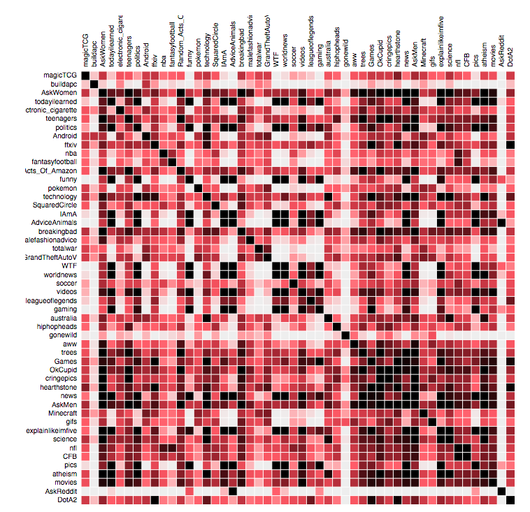
Figure 4. Subreddit word use similarity visualized using an adjacency matrix
One of the most comprehensive methods of display is the adjacency matrix. [37] This method satisfies the condition of showing the relationship of each node to every other one, but it does so at the cost of easy or intuitive decipherability.
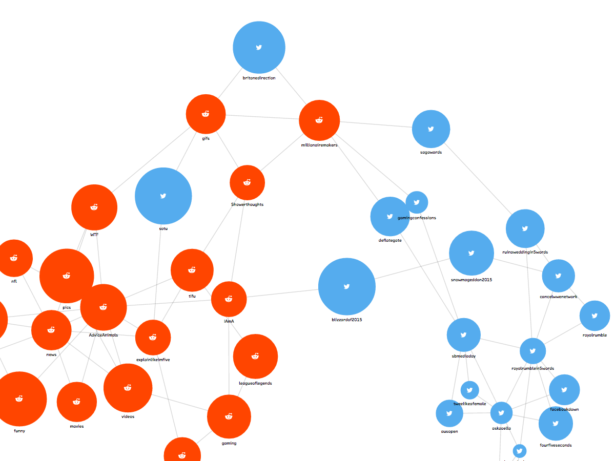
Figure 5. Force-directed graph: the final product
A force-directed graph displays the same information, but it uses humankind’s inherent understanding of physical forces to build a more intuitive model of relationships. [38] The D3.js force-directed layout includes a simplified but robust set of simulated forces based on charged particles and springs. Nodes are pulled toward each other by links according to the strength of their relationship. At the same time, nodes repel one another by a set force (otherwise, the result would be a clump of nodes stacked on top of each other — not a particularly useful visualization). The final visualization is a result of these forces settling into an equilibrium.
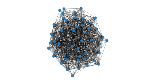
Figure 6. Force-directed graph: the hairball
Force-directed graphs carry their own disadvantages, however. Plugging our data directly into the visualization without any adjustments resulted in a “hairball” effect, in which the number of crossed links overwhelmed any ability to discern meaningful relationships. We first attempted to control the hairballness by creating a link value threshold, removing links whose similarity values were below a certain number. This helped, but because of the variation in size between the subreddits we were examining, the global threshold created a technically correct but ultimately uninformative split between the top and bottom ends of the subreddit size spectrum, where the top nodes still hairballed and the bottom nodes were set adrift.
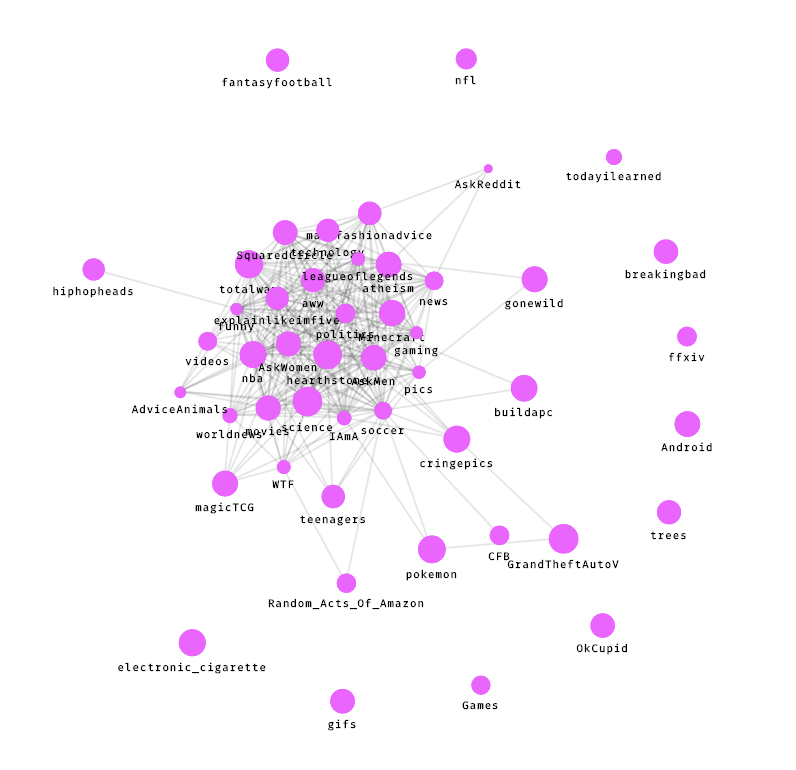
Figure 7. Subreddit word use similarity visualized using a force-directed graph with a global link threshold
What we really needed was a localized threshold, which highlighted each particular node’s strongest links. After a bit of exploration, we settled on the following code, which ensures that each node’s two strongest links are on the graph.
Example 1. Localized threshold for links
// Sort all links from server by strength
raw_links.sort(compareJaccard);
// Loop through those links
for (var i=0; i<raw_links.length; i++) {
  var link = raw_links[i];
  // Get source and target nodes from link
  var source_node = link.source_node;
  var target_node = link.target_node;
  // Set link limit per node
  var limit = 2;
  // If either the source node OR the target node has less than the link limit, then add the link to the graph. This means that each node will have at least the link limit, and many will have more.
  if (source_node.related_nodes.length < limit || target_node.related_nodes.length < limit) {
    source_node.related_nodes.push(link);
    target_node.related_nodes.push(link);
    links.push(link);
  }
}
Because one node’s strongest link could be another’s fifth-strongest, this does not mean each node has only two links, but rather guarantees that each one meets that minimum. We found that this filter, by significantly trimming down the hairball, did a much better job of making the significant links visible and the overall network structure understandable. The type of filter you may want to apply depends, like your data structure, on what questions you are interested in.
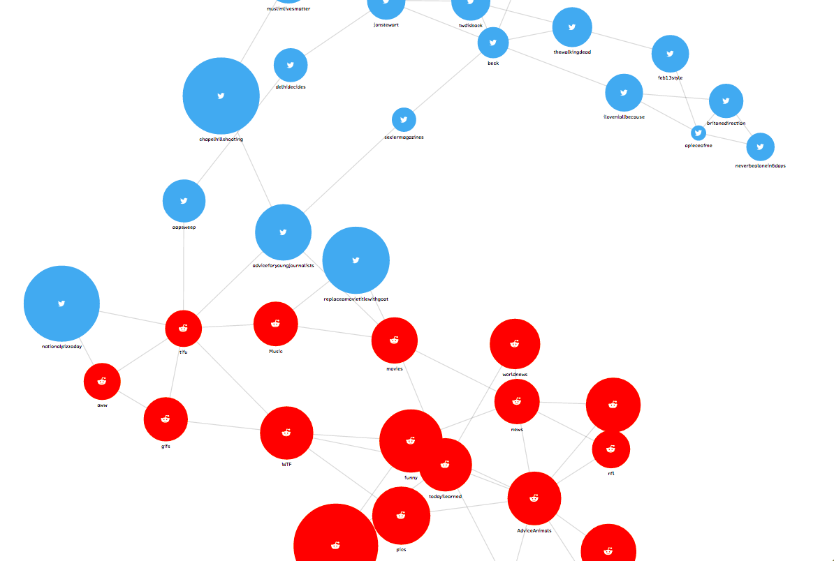
Figure 8. Force-directed graph, with the filter applied
Even with the filter applied, the graph of keyword similarity is still a lot of information to take in. Fortunately, since we are working in an interactive medium, we can let the user clarify their picture of the data through exploration. Using conventions from other visualizations, such as the pan and zoom of Google Maps, makes this process feel intuitive and approachable. In our prototype, hovering over a node highlights its connections while fading the rest of the graph into the background. Clicking on that node pins it to the center and reveals additional information.
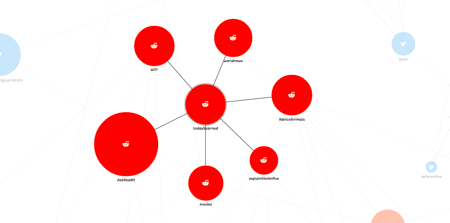
Figure 9. Force-directed graph, node detail
Allowing the user to move through different levels of detail and abstraction helps make the large amount of data in CliqueStream digestible. As our ability to analyze huge amounts of data increases, we must make sure to place an equal focus on making that analysis understandable. Visualizations like force-directed layouts can be a great aid in this process, provided we use them thoughtfully and always as a means to communicate specific information.
Things to Consider
There are many lessons to be learned when creating a streaming data infrastructure and analysis routines. Making mistakes with the initial setup can negatively impact the adoption of these systems if there is a steep learning curve, or create many hidden costs if the infrastructure is inefficient. However, when properly created, an easy data infrastructure can make prototyping new projects and accessing necessary data incredibly easy and reduce the possible complexity (and cost) of the resulting systems.
Special care must also be taken when implementing a streaming analysis application. Streaming data consumers are different from other analysis applications in that they do not stop — as opposed to batch analysis programs that run over a given chunk of data and then stop, streaming programs should be able to keep running as long as there is data to be processed. As a result, special care must be given to architecting in these solutions and understanding how they will operate over time.
Streaming Infrastructure
-
Data should be organized and easy to find.
-
Naming is everything. It should be easy to find and connect to a stream that contains information you will need.
-
Having a directory of all available data is critical to promoting data usage and adoption. NSQ’s nsqadmin application is fantastic for this.
-
-
Data schema should be regular and documented.
- Keys for data should be regular and easily decipherable. All data in the same stream should have the same key values.
-
Decouple data production and consumption.
-
Make sure your streams are queued, fault tolerant, and robust.
-
Upstream services should not be affected if a downstream application fails.
-
If the amount of data created increases past the consumption rate, stream boxes should queue messages (potentially to disk to avoid running out of memory) and alert so that more consumption capacity can be added.
-
Data should be requested from the consumer as opposed to pushed from the data queue. This will keep the consumer insulated and avoid adding more burden to an application that may be experiencing problems.
-
Make sure to have exponential backoffs when experiencing problems and adequate backpressure so that faults do not propagate through the system.
-
-
Think of data availability as guarantees.
-
How much latency can you guarantee between data production and consumption?
-
Can you guarantee that every message will get delivered? What are the bounds on how many times a message can be delivered?
-
Does a consumer get messages it missed if it went offline? What if it went offline for days?
-
Can you guarantee that data will maintain the same schema? Will changes to the data be in a new stream or must clients be able to accept changes?
-
Data Analysis
-
Enumerate the questions being asked by a project and the smaller questions that must be answered along the way.
-
Are these questions providing the insights that are necessary?
-
Can the questions be simplified? Are there other questions that would provide similar insights?
-
How accurate must the answers be to still be useful? Most of the time approximate and order-of-magnitude results are sufficient!
-
-
What are the memory bounds of this solution?
-
How much memory will be needed to do the calculation currently?
-
How much memory will be needed to do the calculation in a year?
-
If the amount of data doubles, what will happen to memory use? How can this be mitigated as resource usage exceeds server capacity? (Increasing server capacity should be a last resort!)
-
-
What are the computational bounds of this solution?
-
How much computation must be done per piece of data?
-
How does computation scale if the data doubles?
-
Can the computation be distributed to many servers? If inter-server communication is necessary for this, how can it be minimized?
-
-
Protect against data outages.
-
What happens if the data stream temporarily stops as a result of upstream problems?
-
Will it take time for the system to recover from problems with upstream data? How long?
-
-
How can you provide the results of your analysis to users or other applications for further processing?
-
Is it worthwhile to output a new stream resulting from your application’s analysis?
-
What is the simplest way to make an API for users to query the current results? What are the most requested results, and how can those be provided easily?
-
What request rate can your application maintain to its API? What happens when this is doubled? Can you use caching to improve this?
-
State of the Industry
There’s been significant growth in recent years in the number of software systems available for working with streaming data, both in the open source and commercial markets. In this section, we review the options currently available for working with data streams, with a focus on implementations of probabilistic algorithms.
Realistically, however, we have found that while there are commodity systems for working with streams of data, very few are designed for probabilistic modeling. Most existing systems are designed to feed realtime data into a traditional SQL database or data warehouse.
Also, the vocabulary commonly used in the market is still evolving. You may see streaming systems referred to as “event processing systems,” or “complex event processing” or even “event correlation” systems. We are starting to see the rich history of legacy event processing systems collide with the modern reality of commoditized Hadoop and other map-reduce infrastructures.
It’s an exciting time for streaming infrastructure, as these tools are beginning to hit maturity and become stable platforms.
Open Source
Much of the impressive development of streaming infrastructure has come from the open source community. There are several projects that are commonly found in production on “web-scale” products. On the business side, several of these projects have large commercial efforts behind them and are great options for enterprise systems.
A product is considered to be “web scale” when it must manage data from very large numbers of Internet users or web pages. The obvious examples are Google and Facebook, but there are many smaller companies that have built impressive infrastructures for managing data.
We have chosen to write about only those open source projects that are proven to work well in production for large-scale systems, and that offer value for probabilistic algorithms. This list is by no means exhaustive; keep in mind also that this is a rapidly evolving field.
Apache Storm
Storm is designed to do for realtime stream processing what Hadoop did for batch processing — that is, create a stable and robust commodity open source solution for a problem area that usually requires messy and complex homebrewed architecture, or very expensive proprietary software.
Storm originated at BackType, a startup founded in 2008 with a focus on providing analytics for businesses across social and web platforms. Work on Storm began in 2010, and the system was open-sourced after Twitter acquired BackType in 2011. It became an official Apache project in 2013.
Practically, Storm is considered by many engineers to be a heavyweight solution. It must also be deployed alongside other infrastructure (Storm only provides the stream management system), so it is not, by itself, a complete solution.
Storm famously powers Twitter’s realtime analytics,[39] and YieldBot has used Storm, alongside Apache Kafka (a distributed messaging system) and Apache Cassandra (a distributed database), for probabilistic ranking and trend analysis.
NSQ and Messaging Protocols
NSQ is a realtime distributed messaging platform that is horizontally scalable and handles high-throughput streams. NSQ is written in Go, a programming language created by Google with strong support for concurrency that is starting to be adopted by many distributed system engineers.
NSQ was developed in 2012 at bitly, a social media analytics company, to handle a messaging architecture that powers many downstream services with varying requirements. It is now running in production at many companies, including Stripe, BuzzFeed, Digg, and Hailo.

Figure 1. NSQ System Architecture
We include NSQ in this review because it is an excellent package for handling incoming data streams that feed into probabilistic systems.
Streamtools
Streamtools[40] is a graphical tool for visually working with streams of data. It was developed in 2013 by the New York Times R&D Lab with the goal of enabling developers to easily work with streams of data.
Streamtools offers a visual vocabulary of operations that can be applied to realtime streams of data without programming. It’s significant because it democratizes the ability to work with realtime streams, vastly increasing the number of people in a typical organization who can create products or find insights on the available data.
RethinkDB
RethinkDB[41] is an emerging project we find fascinating enough to include in this report. It’s an open source distributed database with a built-in administrative interface and intuitive query language.
The RethinkDB team recently added a streaming API that supports working with, querying, and storing realtime streams of data. This feature allows application developers to invert the typical model of development, so that rather than constantly polling a datastore, they can subscribe to database updates and have RethinkDB push those updates into the application. This can be a strong advantage for applications built on realtime data.
Commercial Vendors
Commercial complex event processing systems have been in the market since the 1990s, and all major database vendors offer a streaming data processing solution. These solutions are available at high cost (typical pricing is approximately US$40,000 annually) and are generally only a recommended option if you already run data solutions from a particular vendor in your environment.
The largest difference between the open source options in this space and the commercial ones is the developer experience. All of the commercial options have a recommended or required Integrated Development Environment (IDE). This simplifies the process of integrating streaming analytics into an existing infrastrcture, but forces compliance to a specific metaphor of data flow design.
Few of the provided components use probabilistic models, though implementation is straightforward with any of them.
In this section, we give a brief overview of some of the dominant commercial solutions.
SAP Event Stream Processor (ESP)
The SAP ESP solution includes an Integrated Development Environment (IDE) with a graphical interface to visually connect and program the data sources and outputs. It supports visual analytics, allowing for both realtime and batch analytics to be designed in the same dashboard view.

Figure 2. A screenshot of the SAP ESP analytics design view
IBM InfoSphere Streams
IBM’s offering retails at $43,700.00 for a production annual license. It also offers a graphical view of how data flows through the application (one of their training manuals insists this is the “natural way to view an application”), and allows programmers to use various analysis metaphors for working with and analyzing their data.
Many applications of IBM’s offering are found in the finance industry.
Oracle Event Processing
Oracle’s Event Processing solution is a stand-alone stream processor that also integrates with Oracle’s suite of solutions. It offers a visual data flow editor in the IDE, as well as a web view.
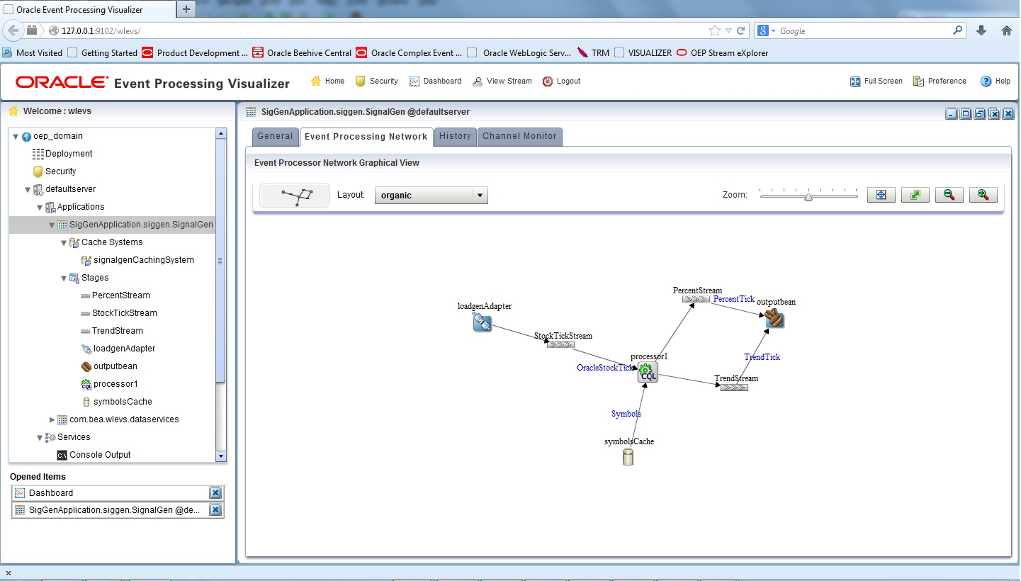
Figure 3. A screenshot of the Oracle Event Processing interface
The Future
Probabilistic methods are putting our current algorithms in a new light — rather than constantly trying to improve their speed by adding more computing power, we can simply allow for a bounded amount of error and get immense gains. This will allow us to move our analyses from the large computing clusters in which they currently reside into the hands of individuals.

Figure 1. Faster and lower resource analysis will bring complex computation to user devices
One potentially very exciting application would be the ability to take in all the sensor data we can get hold of and do very cheap calculations with that data. For example, a fitness tracker could record all available data and provide the user with insights into that data on the device, without the need for a cloud-backed cluster. This is in stark comparison to current approaches, where data is heavily truncated before being sent to a centralized server in the cloud for processing and analysis. The move toward fog computing, where processing, storage, and analysis are done on consumer devices closer to the network edge brings analysis and insights closer to where they should be — with the people asking the questions — so the information is in the right place at the right time. In addition, since the data being analyzed is hashed, the original information is lost and the users can rest assured that their information remains private.
Another point of interest is the ability of these algorithms to deal with changes in the underlying dataset. This is incredibly important as we collect more data, but still care about actionable information that relies on what is happening right now. Incoming data may change completely, and we can accommodate this by using time-windowed versions of the algorithms or, if the change is fundamental to the data type, a change in hash function. Windowed algorithms are not only beneficial in allowing us to bound resource usage, but also provide enhanced understanding of the data by “forgetting” older information and always providing us with the most recent insights.
This ability to window data and, in general, to be able to peek inside of the data structure’s internal state at any point to get the current results is incredibly important in today’s dynamic world. Getting results too late or ones that potentially incorporate data that is of no use anymore lessens the potential impact our results can make. For example, if we were analyzing traffic patterns on our website in relation to changes we have made to content (through A/B testing, or if new content has recently been made available), we would want to know immediately what effect the changes have made. Knowing that most of the readers of the new content also liked another piece of content, or are also users of a particular site feature, or how they compare to other users is extremely actionable information that can be used to greatly enhance user participation and the user experience. Furthermore, in a world where the vast majority of interaction with a new piece of content happens in the first 15 minutes, [42] we do not have time to do anything but a very fast realtime analysis — by the time a batch analysis is done it is already too late!
Finally, probabilistic streaming methods provide a cultural paradigm shift for data analysts. Currently, their job is over once they have an algorithm that is able to output the analysis that they wanted. These methods, however, show themselves as the additional step of cementing the insights they learned in their exploration into systems to make people smarter by answering their questions as they are being asked.
Ethics
One major advantage of probabilistic methods is that they discard the original data in favor of an internal summary (also known as a “sketch” of the original data, or a “synopsis”). This summarization is generally created using a one-way hashing function that makes it almost impossible to reproduce the original data. As a result, almost perfect privacy regarding the original data is guaranteed.
Data breaches are becoming more and more common. Howev- er, if aggregated hashed data is stolen, it’s not currently possi- ble to reverse engineer the source data from the values stored by probabilistic systems (and it’s unlikely to ever be possible with any sort of precision).
For example, we can create a graph that compares cookies of people who go to various websites. We can easily determine how similar the audiences of various websites are, and even analyze the paths by which users navigate through the various resources. However, we cannot give an enumerated list of the cookies that are following these trends (only information regarding how many of them each website has seen, how many are shared between sites, and how many are different). This is the holy grail of bulk analysis — while we can still perform the analysis we require and give in-depth insights regarding user patterns, we cannot identify the users, and we maintain their privacy. This is particularly important when dealing with medical or student data, where laws mandate a level of privacy that often makes analysis more cumbersome.

Figure 2. Probabilistic data structures offer inherit privacy while still allowing for interesting insights in the aggregate
This added anonymity is not only important for the trust of users but it is also becoming more and more legally required as more and more nations legislate for personal data privacy. In the European Union, the Data Protection Directive and the General Data Protection Regulation limit what sort of personally identifiable information may be collected, how it can be used, and how it can cross borders. This has become such a problem that new datacenters are being created in Lithuania, simply as a place within EU borders to perform user analysis. Similarly, in the US user data is protected under HIPAA and various state laws. This has also led to special datacenters (most notably the Amazon AWS HIPAA-compliant servers) specifically designed to easily create a space for compliant analysis.
As a result, there is a fantastic compromise between the needs of service users and organizations interested in deriving insights. Users can provide completely anonymized data with mathematical assurances that their original data cannot be recovered. However, the organizations are still able to derive insights that they are interested in by using the appropriate probabilistic algorithms.
Conclusion
Probabilistic methods give us the ability to perform calculations faster and with fewer resources than previously possible. As large-volume data streams become more ubiquitous, being able to do complex calculations quickly will become increasingly important. With data collection rates continuing to increase, the calculation methods we are currently comfortable with will begin to require overwhelming computational resources. These techniques also open up new potential analysis and product opportunities.
In this report we’ve explored the methods and advances in the field of probabilistic algorithms in order to outline how powerful these algorithms are and how critical they will be in shaping the future of computing. We explained probabilistic algorithms, gave historical context, and provided examples of many common applications which can easily be shaped by these methods, including realtime trend analysis on social networks (as illustrated by our prototype, CliqueStream) and anomaly detection in security.
With the prototype we show the simplification of a complex problem with probabilistic methods. While it was once simply unfeasible to do a similarity graph with the massive dataset containing every word used on Reddit and Twitter, probabilistic algorithms make it possible to do the calculations in realtime using modest computers. In fact, the initial view of the prototype performs a probabilistic calculation in seconds, while it would have taken over 15 minutes to do the equivalent calculation with classical deterministic algorithms. This is a simple demonstration of the power of this approach to working with realtime data.
In addition to allowing us to do classical computations on smaller hardware, the computational edge afforded by probabilistic methods will allow us to change the ways which users interact with algorithms. Since calculations can be done on commodity hardware, even on cell phones, we can bring the algorithms to users and help them get the insights they need immediately and without being tied to a cumbersome cloud architecture. This not only saves on the computational requirements needed for a given service, affords users the privacy that they desire, and opens up new opportunities to create businesses and services that push computation onto the devices themselves.

Figure 1. Probabilistic methods will allow personal devices to be less reliant on cloud architecture
We remain excited about these types of probabilistic systems. There are many applications where these methods can be plugged in today with immediate returns, and even more where they enable novel architectures, allowing for new types of applications. Understanding these methods will unlock new possible insights, turn decision making into a quicker and more data-driven process, and enable new kinds of products to be built.
In 2010, updates about pop star Justin Bieber were believed to consume about 3% of Twitter’s server infrastructure (http://mashable.com/2010/09/07/justin-bieber-twitter/). ↩︎
Thanks to Gary King for this analogy (http://bit.ly/1zxaQit) ↩︎
The complexity might increase, for example, if the number of edges in the graph being analyzed increases. ↩︎
http://en.wikipedia.org/wiki/Histogram#Number_of_bins_and_width ↩︎
These numbers come from the 66-95-99 rule of Gaussian distributions. More information can be found at http://en.wikipedia.org/wiki/68–95–99.7_rule. ↩︎
A more fully fleshed out implementation that uses an array of bytes to make many counters is available at https://github.com/ianozsvald/morris_counter." ↩︎
More information about the error behavior can be seen at http://geomblog.blogspot.co.uk/2011/06/bob-morris-and-stream-algorithms.html. ↩︎
Beyer, K., Haas, P. J., Reinwald, B., Sismanis, Y., and Gemulla, R. “On synopses for distinct-value estimation under multiset operations.” Proceedings of the 2007 ACM SIGMOD International Conference on Management of Data - SIGMOD ’07 (2007): 199-210. doi:10.1145/1247480.1247504. ↩︎
Bloom, B. H. “Space/time trade-offs in hash coding with allowable errors.” Communications of the ACM 13:7 (1970): 422-426. doi:10.1145/362686.362692. ↩︎
The Wikipedia page on Bloom filters has a very simple proof for the properties of a Bloom filter; see http://en.wikipedia.org/wiki/Bloom_filter#Probability_of_false_positives. ↩︎
Almeida, P. S., Baquero, C., Preguiça, N., and Hutchison, D. “Scalable Bloom Filters.” Information Processing Letters 101 (2007): 255–261. doi:10.1016/j.ipl.2006.10.007. ↩︎
The error values actually decrease like the geometric series. This way, when you take the product of all the error rates it approaches the desired error rate. ↩︎
http://algo.inria.fr/flajolet/Publications/DuFl03-LNCS.pdf ↩︎
A full description of the basic LogLog and SuperLogLog algorithms can be found at http://algo.inria.fr/flajolet/Publications/DuFl03.pdf. ↩︎
Durand, M., and Flajolet, P. “LogLog Counting of Large Cardinalities.” Proceedings of ESA, 2832 (2003): 605-617. doi:10.1007/978-3-540-39658-1_55. ↩︎
Flajolet, P., Fusy, É, Gandouet, O., et al. “HyperLogLog: The analysis of a near-optimal cardinality estimation algorithm.” Proceedings of the International Conference on Analysis of Algorithms (2007): 127–146. ↩︎
Spherical averaging is simply a more complicated statistical measure that relates to the normal average. ↩︎
Union operations occur without increasing the error rate. ↩︎
Size of data structure with 0.05% error rate, 100,000,000 unique elements, and using a 64-bit hashing function. ↩︎
These operations can be done ↩︎
Processing time has been adjusted to remove the time required to read the dataset from disk. We also use the simple implementations provided earlier for testing. ↩︎
Structure size is theoretical given the amount of data since the implementations used were not optimized. ↩︎
Since the Morris counter doesn’t deduplicate input, the size and relative error are given with regard to the total number of values. ↩︎
Because of some encoding problems, the datrie could not load all the keys. ↩︎
The dataset is 49,558 KB considering only unique tokens, or 8.742 GB with all tokens. ↩︎
Virtual reality systems may soon offer new opportunities for more immersive data visualizations, but we’ll still be short by 37 dimensions. ↩︎